Data#
Independently of the model, data will be needed for either creating or validating the model. The amount of data required will be determined by a trade-off between complexity-affordability-accuracy , and the type of model. Data-driven models will likely require a broad range and large volume of data, while mechanistic models may only need data for a defined set of variables.
1.1 Data Sources#
Berkeley Earth Global Temperature
Daily average temperature observations
Resolution 1° x 1°
Monthly mean temperature FAIRBANKS
80 km from Nenana, data from 1828 - 2020
Monthly mean temperature HEALY RIVER AIRPORT
90 km from Nenana, data from 1983 - 2012
Monthly mean temperature MOUNT MCKINLEY NATL
100 km from Nenana, data from 1923 - 2013
NOAA GHCN: Nenana
NOAA GHCN: Fairbanks
USGS Water Data: Nenana
USGS Water Data: Fairbanks
USGS Water Data: Fairbanks
NERC-EDS Global Cloud Coverage
TEMIS Global Solar Surface Irradiance
USGS Glaciers Data: Gulkana
NOAA Global Indexes
Nenana Ice Classic
Ice thickness measurements
Ice break up dates
1.2 Loading data#
If you are new to Python you are probably aware of some basic data structures like lists and dictionaries, maybe even NumPy arrays.
We will now introduce a new data structure, DataFrames.
DataFrames#
A DataFrame is tabular data structure that stores information in rows and columns, where each column has a name and can hold different types of data. Both the rows and columns can have labels, making it easier to access and manipulate specific part of the data (very colloquially, think of a dataframe as a mix between dictionaries and a spreadsheets)
In Python, we will use Pandas.Dataframes (quick introduction)
DataFrames are particularly useful because we can easily manipulate data using a wide variety built-in methods. Additionally, pandas.dataframe can easily handle data with timestamps, meaning, that we can assign a date and time to each observation and manipulate these variables without worrying about time zones, leap years, or other time-related issues. For example, you can subtract one date from another to find the number of days between them, access data for specific years or months, iterate through years, etc.
In addition to rows and columns, dataframe have an .index.The index is series of labels associated to each row, by default the index assign an integer, starting from 0, to each row.
When working with time-series it may be convenient to use a DatetimeIndex to assign a timestamp label to each row instead.
Task 1:
The files corresponding to the sources mentioned above are available in the repository in the folder data/raw_files, choose a file, load the contents to a Pandas.DataFrame, set the index to a datetime object and plot the timeseries.
Tips/Help
Read the documentation for pd.read_csv. Pay special attention to the following methods and arguments
pd.read_csv()
skip_row
sep
index_col
pd.index=pd.to_datetime()format
If you downloaded this notebook, you will need to download the file from the repository and pass the filepath to pd.read_csv.
If you cloned the whole repository, the data files can be easily loaded using the relative path ../../data/raw_files/file_name.txt
If you are running the notebook in your browser, use the function import_data_browser from the ice package to load the file into the browser. The function needs the URL of the file within the repository, specifically the raw URL. To obtain this, navigate to the file in the repository, and in the upper right-hand side, there is a button named Raw that will direct you to a page with the raw contents of the text file. The URL of this page is the URL that you need to pass to the function.
# EX 1.
# # Exercise 1.

import pandas as pd
import matplotlib.pyplot as plt
import iceclassic as ice


#Temp=pd.read_csv('../../data/raw_files/Berkeley temp.txt',skiprows=23,sep='\t',index_col=0)
file1=ice.import_data_browser('https://raw.githubusercontent.com/iceclassic/mude/main/book/data_files/Berkeley%20temp.txt')
Temp=pd.read_csv(file1,skiprows=23,sep='\t',index_col=0)

Temp.index=pd.to_datetime(Temp.index,format='%Y%m%d')

plt.figure(figsize=(20,5))
plt.plot(Temp)
plt.title("Temperature Data")
plt.xlabel("Date")
plt.ylabel("Temperature (C)")
plt.show()
Task 2:
Choose another file, load it and merge it to the previously loaded file, make sure that the resulting DataFrame contains two columns and a datetime index.
Tips/Help
Read the documentation for pd.merge.
If we merge two dataframe (df1, df2) with datetime indexes, the observations (rows) kept in the resulting dataframe depend on the type merge, this is determine by the argument how.
- `how='inner'`: Only observation associted with dates present in both df1 and df2 are kept.
- `how='left'`:  All observation from df1 are kept. Observation in df2 with dates that don’t match dates in df1 are filled with NA.
- `how='right'`: Similar to `how='left'`, but observations from second df are kept.
- `how='outer'`: All observation from both df1 and df2 are kept. Observation associated with non-matching dates are filled with NA.
# # Exercise 2.
# Loading 2nd file

#PDO=pd.read_csv('../../data/raw_files/PDO.csv',skiprows=1,index_col=0,sep=';')
file2=ice.import_data_browser('https://raw.githubusercontent.com/iceclassic/mude/main/book/data_files/PDO.csv')
PDO=pd.read_csv(file2,skiprows=1,index_col=0,sep=';')
PDO.index=pd.to_datetime(PDO.index,format='%Y%m')

# Merging
merged=pd.merge(Temp,PDO,left_index=True,right_index=True,how='outer')
merged.info()
<class 'pandas.core.frame.DataFrame'>
DatetimeIndex: 46500 entries, 1854-01-01 to 2020-02-01
Data columns (total 2 columns):
 #   Column                                     Non-Null Count  Dtype
---  ------                                     --------------  -----
 0   # TAVG [degree C] Air Surface Temperature  46018 non-null  float64
 1   Value                                      1994 non-null   float64
dtypes: float64(2)
memory usage: 1.1 MB
1.3 Basic DataFrame manipulation#
The function pd.read_csv can loading most data files. However, dealing with files with varying use of separators, delimiters, data types and formats can be a time-consuming.
To simplify the process of loading and merging multiple DataFrames individually, all data sources have been merged into a single text file that can be easily loaded. The file can be found in data/Time_series_DATA.txt
The file has more than 20 variables (columns), some of which have daily observations spanning more than a century. To contextualize this variable the following interactive map shows the weather station where they were measured.
upload the files to github for this map, as the functions allows to choose the detail level we need a bunch of shapefiles
#ice.plot_interactive_map(plot_only_nearby_basin=False)
---------------------------------------------------------------------------
DataSourceError                           Traceback (most recent call last)
Cell In[5], line 1
----> 1 ice.plot_interactive_map(plot_only_nearby_basin=False)

File c:\Users\gabri\anaconda3\envs\ice_package_test\Lib\site-packages\iceclassic\example.py:1180, in plot_interactive_map(Pfafstetter_levels, plot_only_nearby_basin)
   1178 # changing the level to higher number yield more basin, using Pfafstetter levels 1-12 source HydroBASINS
   1179 file='../../data/shape_files/hybas_lake_ar_lev'+'{:02d}'.format(Pfafstetter_levels)+'_v1c.shp'
-> 1180 gdf_basin_lev = gpd.read_file(file)
   1181 if plot_only_nearby_basin:
   1182     if Pfafstetter_levels==1:

File c:\Users\gabri\anaconda3\envs\ice_package_test\Lib\site-packages\geopandas\io\file.py:294, in _read_file(filename, bbox, mask, columns, rows, engine, **kwargs)
    291             from_bytes = True
    293 if engine == "pyogrio":
--> 294     return _read_file_pyogrio(
    295         filename, bbox=bbox, mask=mask, columns=columns, rows=rows, **kwargs
    296     )
    298 elif engine == "fiona":
    299     if pd.api.types.is_file_like(filename):

File c:\Users\gabri\anaconda3\envs\ice_package_test\Lib\site-packages\geopandas\io\file.py:547, in _read_file_pyogrio(path_or_bytes, bbox, mask, rows, **kwargs)
    538     warnings.warn(
    539         "The 'include_fields' and 'ignore_fields' keywords are deprecated, and "
    540         "will be removed in a future release. You can use the 'columns' keyword "
   (...)
    543         stacklevel=3,
    544     )
    545     kwargs["columns"] = kwargs.pop("include_fields")
--> 547 return pyogrio.read_dataframe(path_or_bytes, bbox=bbox, **kwargs)

File c:\Users\gabri\anaconda3\envs\ice_package_test\Lib\site-packages\pyogrio\geopandas.py:261, in read_dataframe(path_or_buffer, layer, encoding, columns, read_geometry, force_2d, skip_features, max_features, where, bbox, mask, fids, sql, sql_dialect, fid_as_index, use_arrow, on_invalid, arrow_to_pandas_kwargs, **kwargs)
    256 if not use_arrow:
    257     # For arrow, datetimes are read as is.
    258     # For numpy IO, datetimes are read as string values to preserve timezone info
    259     # as numpy does not directly support timezones.
    260     kwargs["datetime_as_string"] = True
--> 261 result = read_func(
    262     path_or_buffer,
    263     layer=layer,
    264     encoding=encoding,
    265     columns=columns,
    266     read_geometry=read_geometry,
    267     force_2d=gdal_force_2d,
    268     skip_features=skip_features,
    269     max_features=max_features,
    270     where=where,
    271     bbox=bbox,
    272     mask=mask,
    273     fids=fids,
    274     sql=sql,
    275     sql_dialect=sql_dialect,
    276     return_fids=fid_as_index,
    277     **kwargs,
    278 )
    280 if use_arrow:
    281     meta, table = result

File c:\Users\gabri\anaconda3\envs\ice_package_test\Lib\site-packages\pyogrio\raw.py:196, in read(path_or_buffer, layer, encoding, columns, read_geometry, force_2d, skip_features, max_features, where, bbox, mask, fids, sql, sql_dialect, return_fids, datetime_as_string, **kwargs)
     56 """Read OGR data source into numpy arrays.
     57
     58 IMPORTANT: non-linear geometry types (e.g., MultiSurface) are converted
   (...)
    191
    192 """
    194 dataset_kwargs = _preprocess_options_key_value(kwargs) if kwargs else {}
--> 196 return ogr_read(
    197     get_vsi_path_or_buffer(path_or_buffer),
    198     layer=layer,
    199     encoding=encoding,
    200     columns=columns,
    201     read_geometry=read_geometry,
    202     force_2d=force_2d,
    203     skip_features=skip_features,
    204     max_features=max_features or 0,
    205     where=where,
    206     bbox=bbox,
    207     mask=_mask_to_wkb(mask),
    208     fids=fids,
    209     sql=sql,
    210     sql_dialect=sql_dialect,
    211     return_fids=return_fids,
    212     dataset_kwargs=dataset_kwargs,
    213     datetime_as_string=datetime_as_string,
    214 )

File c:\Users\gabri\anaconda3\envs\ice_package_test\Lib\site-packages\pyogrio\_io.pyx:1239, in pyogrio._io.ogr_read()

File c:\Users\gabri\anaconda3\envs\ice_package_test\Lib\site-packages\pyogrio\_io.pyx:219, in pyogrio._io.ogr_open()

DataSourceError: ../../data/shape_files/hybas_lake_ar_lev04_v1c.shp: No such file or directory
Task 3:
Read the documentation of explore_data() from the iceclassic package and use it to explore the contents of Time_series_DATA.txt.
Decide which variables might not be relevant to the problem ? Explain.
#Data=pd.read_csv("../../data/Time_series_DATA.txt",skiprows=149,index_col=0,sep='\t')
file3=ice.import_data_browser('https://raw.githubusercontent.com/iceclassic/mude/main/book/data_files/time_serie_data.txt')
Data=pd.read_csv(file3,skiprows=162,index_col=0,sep='\t')
Data.index = pd.to_datetime(Data.index, format="%Y-%m-%d")
ice.explore_contents(Data)
<class 'pandas.core.frame.DataFrame'>
DatetimeIndex: 39309 entries, 1901-02-01 to 2024-02-06
Data columns (total 28 columns):
 #   Column                                             Non-Null Count  Dtype
---  ------                                             --------------  -----
 0   Regional: Air temperature [C]                      38563 non-null  float64
 1   Days since start of year                           38563 non-null  float64
 2   Days until break up                                38563 non-null  float64
 3   Nenana: Rainfall [mm]                              29547 non-null  float64
 4   Nenana: Snowfall [mm]                              19945 non-null  float64
 5   Nenana: Snow depth [mm]                            15984 non-null  float64
 6   Nenana: Mean water temperature [C]                 2418 non-null   float64
 7   Nenana: Mean Discharge [m3/s]                      22562 non-null  float64
 8   Nenana: Air temperature [C]                        31171 non-null  float64
 9   Fairbanks: Average wind speed [m/s]                9797 non-null   float64
 10  Fairbanks: Rainfall [mm]                           29586 non-null  float64
 11  Fairbanks: Snowfall [mm]                           29586 non-null  float64
 12  Fairbanks: Snow depth [mm]                         29555 non-null  float64
 13  Fairbanks: Air Temperature [C]                     29587 non-null  float64
 14  IceThickness [cm]                                  461 non-null    float64
 15  Regional: Solar Surface Irradiance [W/m2]          86 non-null     float64
 16  Regional: Cloud coverage [%]                       1463 non-null   float64
 17  Global: ENSO-Southern oscillation index            876 non-null    float64
 18  Gulkana Temperature [C]                            19146 non-null  float64
 19  Gulkana Precipitation [mm]                         18546 non-null  float64
 20  Gulkana: Glacier-wide winter mass balance [m.w.e]  58 non-null     float64
 21  Gulkana: Glacier-wide summer mass balance [m.w.e]  58 non-null     float64
 22  Global: Pacific decadal oscillation index          1346 non-null   float64
 23  Global: Artic oscillation index                    889 non-null    float64
 24  Nenana: Gage Height [m]                            4666 non-null   float64
 25  IceThickness gradient [cm/day]: Forward            426 non-null    float64
 26  ceThickness gradient [cm/day]: Backward            426 non-null    float64
 27  ceThickness gradient [cm/day]: Central             391 non-null    float64
dtypes: float64(28)
memory usage: 8.7 MB
Task 4:
The file contains data for three distinct temperature timeseries, use compare_columns to visually compare them.
Then, use .drop() to eliminate the columns that might be redundant .
temperature_columns=['Regional: Air temperature [C]','Nenana: Air temperature [C]','Fairbanks: Air Temperature [C]','Gulkana Temperature [C]']
ice.compare_columns(Data,temperature_columns)
Data=Data.drop(columns=temperature_columns[1:3])
The contents of a DataFramecan be grouped into subsets of the dataframe by means of simple indexing.
There are three main ways to use indexing to create a subset of the dataframe
df.loc[]: uses the label of columns (column names) and rows (index) to select the subsetdf.iloc[]: uses integers indexes to select the subsetdf[]: uses the column name to select the column. Additionally we can pass a list/array of boolean values to use as a mask
Task 5:
Create a new dataframe with a subset containing only the data from 1950 onwards
Data_2 = Data[(Data.index.year >= 1950)]
Data_2.info()
<class 'pandas.core.frame.DataFrame'>
DatetimeIndex: 27065 entries, 1950-01-01 to 2024-02-06
Data columns (total 26 columns):
 #   Column                                             Non-Null Count  Dtype
---  ------                                             --------------  -----
 0   Regional: Air temperature [C]                      26510 non-null  float64
 1   Days since start of year                           26510 non-null  float64
 2   Days until break up                                26510 non-null  float64
 3   Nenana: Rainfall [mm]                              22266 non-null  float64
 4   Nenana: Snowfall [mm]                              13322 non-null  float64
 5   Nenana: Snow depth [mm]                            12965 non-null  float64
 6   Nenana: Mean water temperature [C]                 2418 non-null   float64
 7   Nenana: Mean Discharge [m3/s]                      22562 non-null  float64
 8   Fairbanks: Average wind speed [m/s]                9797 non-null   float64
 9   Fairbanks: Rainfall [mm]                           22250 non-null  float64
 10  Fairbanks: Snowfall [mm]                           22250 non-null  float64
 11  Fairbanks: Snow depth [mm]                         22250 non-null  float64
 12  IceThickness [cm]                                  461 non-null    float64
 13  Regional: Solar Surface Irradiance [W/m2]          86 non-null     float64
 14  Regional: Cloud coverage [%]                       876 non-null    float64
 15  Global: ENSO-Southern oscillation index            876 non-null    float64
 16  Gulkana Temperature [C]                            19146 non-null  float64
 17  Gulkana Precipitation [mm]                         18546 non-null  float64
 18  Gulkana: Glacier-wide winter mass balance [m.w.e]  58 non-null     float64
 19  Gulkana: Glacier-wide summer mass balance [m.w.e]  58 non-null     float64
 20  Global: Pacific decadal oscillation index          889 non-null    float64
 21  Global: Artic oscillation index                    889 non-null    float64
 22  Nenana: Gage Height [m]                            4666 non-null   float64
 23  IceThickness gradient [cm/day]: Forward            426 non-null    float64
 24  ceThickness gradient [cm/day]: Backward            426 non-null    float64
 25  ceThickness gradient [cm/day]: Central             391 non-null    float64
dtypes: float64(26)
memory usage: 5.6 MB
Task 6
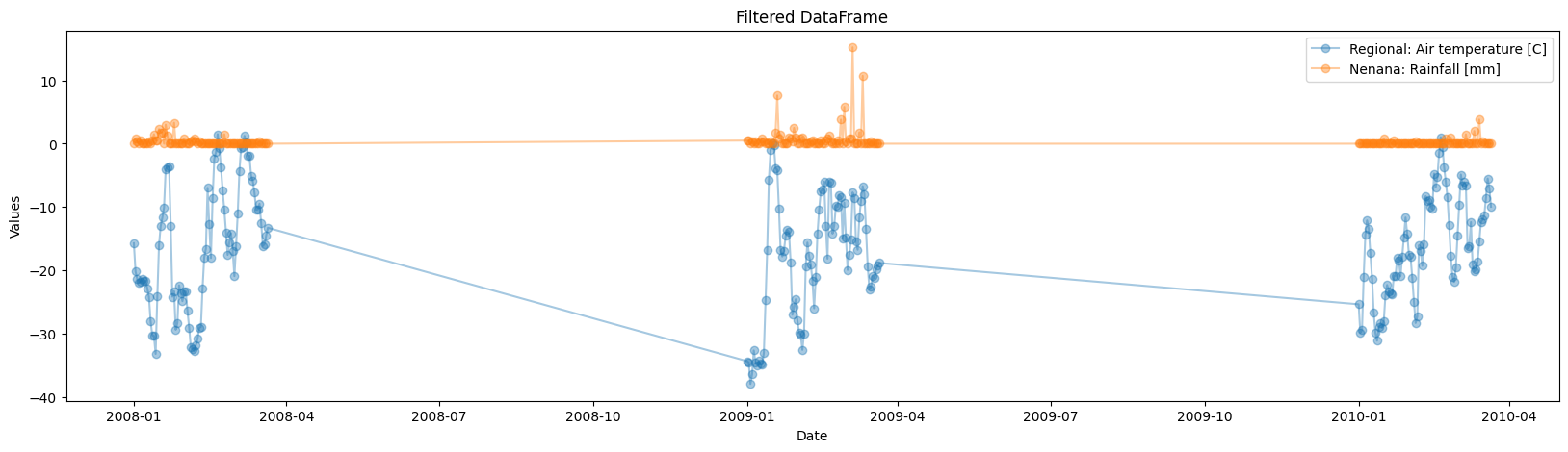
Create a new DataFrame which contains only the columns ['Regional: Air temperature [C]','Nenana: Rainfall [mm]'], for the years [2008,2010], from jan-01 to may-01.
Filter the original DataFrame using masks.
Tips/Help
Use df.index.year to create a mask that filters the years and df.index.strftime() for the mask pertaining to the dates.
cols=['Regional: Air temperature [C]','Nenana: Rainfall [mm]']
years=[2008,2009,2010]
date_1='01/01'
date_2='03/21'

year_mask = Data.index.year.isin(years) # (df.index.year >= min(years)) & (df.index.year <= max(years)) is also an option
date_mask = (Data.index.strftime('%m/%d') >= date_1) & (Data.index.strftime('%m/%d') <= date_2)
filtered_df = Data.loc[year_mask & date_mask, cols]

plt.figure(figsize=(20,5))
plt.plot(filtered_df.index,filtered_df,alpha=0.4,marker='o')
plt.xlabel("Date")
plt.ylabel("Values")
plt.title("Filtered DataFrame")
plt.legend(filtered_df.columns)
plt.show()
1.4 Interactive Plot#
The DataFrame has decades of observations, which causes the xaxis(date) of the plot to lose detail, we could make the figure larger, or plot subset of the dataframe, alternatively we can use plot_columns_interactive() to create a plot were we can scroll and zoom at specific dates.
::{card} Ex 9
Read the documentation for plot_columns_interactive() from the iceclassic package and create an interactive plot.
change the location of the file to the -github path- the function internally uses a file wiht the break up dates, eaither change it or extract this date from the the big dataframe with
break_up_dates=Data.index[Data['Days until break up']==0]
column_groups = {
    'Group 1': ['Regional: Air temperature [C]','Gulkana Temperature [C]'],
    'Group 2': ['Nenana: Snow depth [mm]'],
    'Group 3': ['Nenana: Mean Discharge [m3/s]']}

# Plot the specified columns with default y_domains and focus on a specific date
#ice.plot_columns_interactive(Data, column_groups, title="Break up times & Global Variables at Tenana River-Nenana, AK with break-up dates")