MUDE W3- Gradient Estimation#
Info:
This notebook is a very simple draft showing how we could use data from the ~~Nenana Ice Classic~~ (from any of the column in our dateset) for the numerical modelling part of MUDE.
The implementation is not particularly efficient, but it is quite flexible.
The dataset used is direclty loaded from github, so a a few extra packages are needed(io and requests) but we could avoid using ‘non-standard’libraries by downloading the file and loading it ‘manually’.
from io import StringIO
import requests
import pandas as pd
import numpy as np
import matplotlib.pyplot as plt
import plotly.graph_objects as go
import plotly.express as px
import plotly
import iceclassic as ice
Loading the dataset#
# we could load the data from the repo
file=ice.import_data_browser('https://raw.githubusercontent.com/iceclassic/mude/main/book/data_files/time_serie_data.txt')
Data=pd.read_csv(file,skiprows=162,index_col=0,sep='\t')
Data.index = pd.to_datetime(Data.index, format="%Y-%m-%d")
#Data.info()
River_data=Data[['Nenana: Mean Discharge [m3/s]','Nenana: Gage Height [m]']]
#River_data.info()
River_data.dropna(inplace=True)


Ice_temp=Data[['IceThickness [cm]','Regional: Air temperature [C]']]
Ice_temp.dropna(how='all', inplace=True)
Ice_temp['Day']=Ice_temp.index.dayofyear

Ice_temp.info()
Ice_temp.to_csv('Ice&Temp.csv')
<class 'pandas.core.frame.DataFrame'>
DatetimeIndex: 38578 entries, 1917-01-01 to 2023-04-21
Data columns (total 3 columns):
 #   Column                         Non-Null Count  Dtype
---  ------                         --------------  -----
 0   IceThickness [cm]              461 non-null    float64
 1   Regional: Air temperature [C]  38563 non-null  float64
 2   Day                            38578 non-null  int32
dtypes: float64(2), int32(1)
memory usage: 1.0 MB
C:\Users\gabri\AppData\Local\Temp\ipykernel_13704\1496965268.py:8: SettingWithCopyWarning:
A value is trying to be set on a copy of a slice from a DataFrame

See the caveats in the documentation: https://pandas.pydata.org/pandas-docs/stable/user_guide/indexing.html#returning-a-view-versus-a-copy
  River_data.dropna(inplace=True)
C:\Users\gabri\AppData\Local\Temp\ipykernel_13704\1496965268.py:12: SettingWithCopyWarning:
A value is trying to be set on a copy of a slice from a DataFrame

See the caveats in the documentation: https://pandas.pydata.org/pandas-docs/stable/user_guide/indexing.html#returning-a-view-versus-a-copy
  Ice_temp.dropna(how='all', inplace=True)
C:\Users\gabri\AppData\Local\Temp\ipykernel_13704\1496965268.py:13: SettingWithCopyWarning:
A value is trying to be set on a copy of a slice from a DataFrame.
Try using .loc[row_indexer,col_indexer] = value instead

See the caveats in the documentation: https://pandas.pydata.org/pandas-docs/stable/user_guide/indexing.html#returning-a-view-versus-a-copy
  Ice_temp['Day']=Ice_temp.index.dayofyear
River_data=pd.read_csv('Nenana_River.csv',index_col=0)
River_data.index = pd.to_datetime(River_data.index, format="%Y-%m-%d")
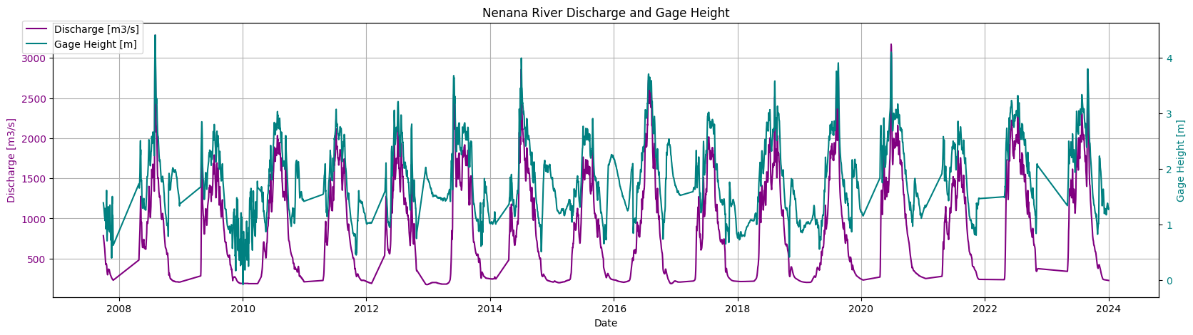
fig, ax1 = plt.subplots(figsize=(20, 5))
ax1.set_title("Nenana River Discharge and Gage Height")
ax1.plot(River_data.index, River_data['Nenana: Mean Discharge [m3/s]'], color='purple', label='Discharge [m3/s]')
ax1.set_xlabel('Date')
ax1.set_ylabel('Discharge [m3/s]', color='purple')
ax1.tick_params(axis='y', labelcolor='purple')
ax1.grid()
# ax1.set_xlim(pd.Timestamp('2018-01-01'), pd.Timestamp('2018-12-31'))
ax2 = ax1.twinx()
ax2.plot(River_data.index, River_data['Nenana: Gage Height [m]'], color='teal', label='Gage Height [m]')
ax2.set_ylabel('Gage Height [m]', color='teal')
ax2.tick_params(axis='y', labelcolor='teal')
fig.legend(loc='upper left', bbox_to_anchor=(0.1, 0.9))
plt.show()
# we could load the data from the repo
file=ice.import_data_browser('https://raw.githubusercontent.com/iceclassic/mude/main/book/data_files/time_serie_data.txt')
Data=pd.read_csv(file,skiprows=162,index_col=0,sep='\t')
Data.index = pd.to_datetime(Data.index, format="%Y-%m-%d")
Data.info()


break_up_dates=Data.index[Data['Days until break up']==0]

print(str(break_up_dates[break_up_dates.year==2019]))
<class 'pandas.core.frame.DataFrame'>
DatetimeIndex: 39309 entries, 1901-02-01 to 2024-02-06
Data columns (total 28 columns):
 #   Column                                             Non-Null Count  Dtype
---  ------                                             --------------  -----
 0   Regional: Air temperature [C]                      38563 non-null  float64
 1   Days since start of year                           38563 non-null  float64
 2   Days until break up                                38563 non-null  float64
 3   Nenana: Rainfall [mm]                              29547 non-null  float64
 4   Nenana: Snowfall [mm]                              19945 non-null  float64
 5   Nenana: Snow depth [mm]                            15984 non-null  float64
 6   Nenana: Mean water temperature [C]                 2418 non-null   float64
 7   Nenana: Mean Discharge [m3/s]                      22562 non-null  float64
 8   Nenana: Air temperature [C]                        31171 non-null  float64
 9   Fairbanks: Average wind speed [m/s]                9797 non-null   float64
 10  Fairbanks: Rainfall [mm]                           29586 non-null  float64
 11  Fairbanks: Snowfall [mm]                           29586 non-null  float64
 12  Fairbanks: Snow depth [mm]                         29555 non-null  float64
 13  Fairbanks: Air Temperature [C]                     29587 non-null  float64
 14  IceThickness [cm]                                  461 non-null    float64
 15  Regional: Solar Surface Irradiance [W/m2]          86 non-null     float64
 16  Regional: Cloud coverage [%]                       1463 non-null   float64
 17  Global: ENSO-Southern oscillation index            876 non-null    float64
 18  Gulkana Temperature [C]                            19146 non-null  float64
 19  Gulkana Precipitation [mm]                         18546 non-null  float64
 20  Gulkana: Glacier-wide winter mass balance [m.w.e]  58 non-null     float64
 21  Gulkana: Glacier-wide summer mass balance [m.w.e]  58 non-null     float64
 22  Global: Pacific decadal oscillation index          1346 non-null   float64
 23  Global: Artic oscillation index                    889 non-null    float64
 24  Nenana: Gage Height [m]                            4666 non-null   float64
 25  IceThickness gradient [cm/day]: Forward            426 non-null    float64
 26  ceThickness gradient [cm/day]: Backward            426 non-null    float64
 27  ceThickness gradient [cm/day]: Central             391 non-null    float64
dtypes: float64(28)
memory usage: 8.7 MB
DatetimeIndex(['2019-04-14'], dtype='datetime64[ns]', freq=None)
Estimating gradients#
the function below its included in the Pypi package, I’ll leave the code here for a while to double check the implementation is correct and I’ll remove it in a few days/week
def finite_differences(series:pd.Series): “”” Computes forward, central, and backward differences using the step size as days between measurement.
Parameters
---------
series: pd.Series
    Series with datetime index

Returns
---------
df: pd.DataFrame
    DataFrame with forward, backward and central differences for the Series

"""

days_forward = (series.index.to_series().shift(-1) - series.index.to_series()).dt.days
days_backward = (series.index.to_series() - series.index.to_series().shift(1)).dt.days

# Forward difference: (f(x+h) - f(x)) / h
forward = (series.shift(-1) - series) / days_forward

# Backward difference: (f(x) - f(x-h)) / h,
backward = (series - series.shift(1)) / days_backward

# Central difference: (f(x+h) - f(x-h)) / (h_forward + h_backward)
central = (series.shift(-1) - series.shift(1)) / (days_forward + days_backward) #

# fixing start/end points
forward.iloc[-1] = np.nan
backward.iloc[0] = np.nan

return pd.DataFrame({'forward': forward, 'backward': backward, 'central': central})
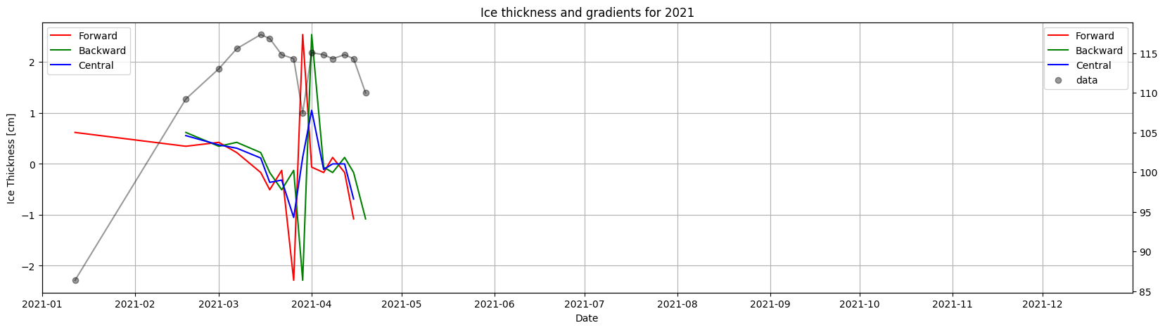
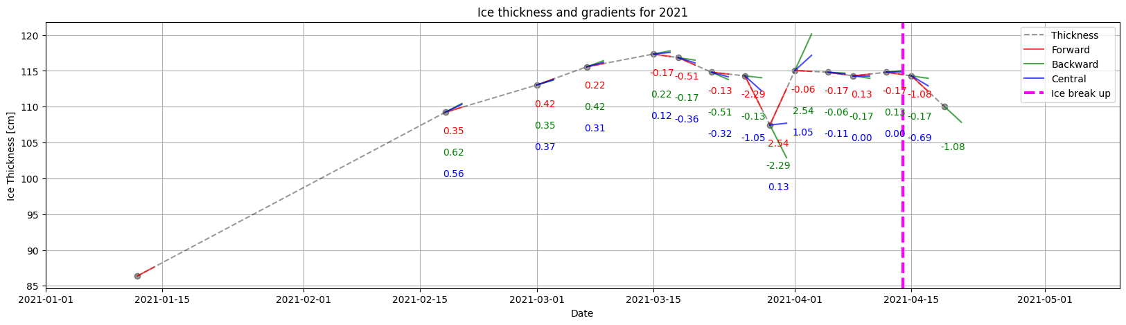
Ice thickness#
Ice_thickness=Data['IceThickness [cm]']
Ice_thickness=Ice_thickness.dropna(inplace=False)
print(Ice_thickness.head())
result = Ice_thickness.groupby(Ice_thickness.index.year,group_keys=True).apply(lambda x: ice.finite_differences(x)).reset_index(level=0, drop=True)

print(result)
ice.plot_gradients_and_timeseries(result,
                             Ice_thickness,
                            2021,
                            Title='Ice thickness and gradients for 2021',
                            ylabel='Ice Thickness [cm]')

ice.plot_gradients_and_timeseries(result,
                            Ice_thickness,
                            year=2021,
                            plot_gradient_as_slope=True,
                            xlim=['01/01', '05/10'],
                            Title='Ice thickness and gradients for 2021',
                            ylabel='Ice Thickness [cm]',
                            vline={'Ice break up': break_up_dates[break_up_dates.year == 2019].strftime('%m/%d')[0]})
1989-02-26    106.68
1989-03-16     95.25
1989-03-21     95.25
1989-03-25    102.87
1989-03-28    105.41
Name: IceThickness [cm], dtype: float64
             forward  backward   central
1989-02-26 -0.635000       NaN       NaN
1989-03-16  0.000000 -0.635000 -0.496957
1989-03-21  1.905000  0.000000  0.846667
1989-03-25  0.846667  1.905000  1.451429
1989-03-28  0.181429  0.846667  0.381000
...              ...       ...       ...
2023-04-07  1.439333 -1.270000 -0.108857
2023-04-10 -0.635000  1.439333  0.254000
2023-04-14  0.000000 -0.635000 -0.362857
2023-04-17  0.190500  0.000000  0.108857
2023-04-21       NaN  0.190500       NaN

[461 rows x 3 columns]
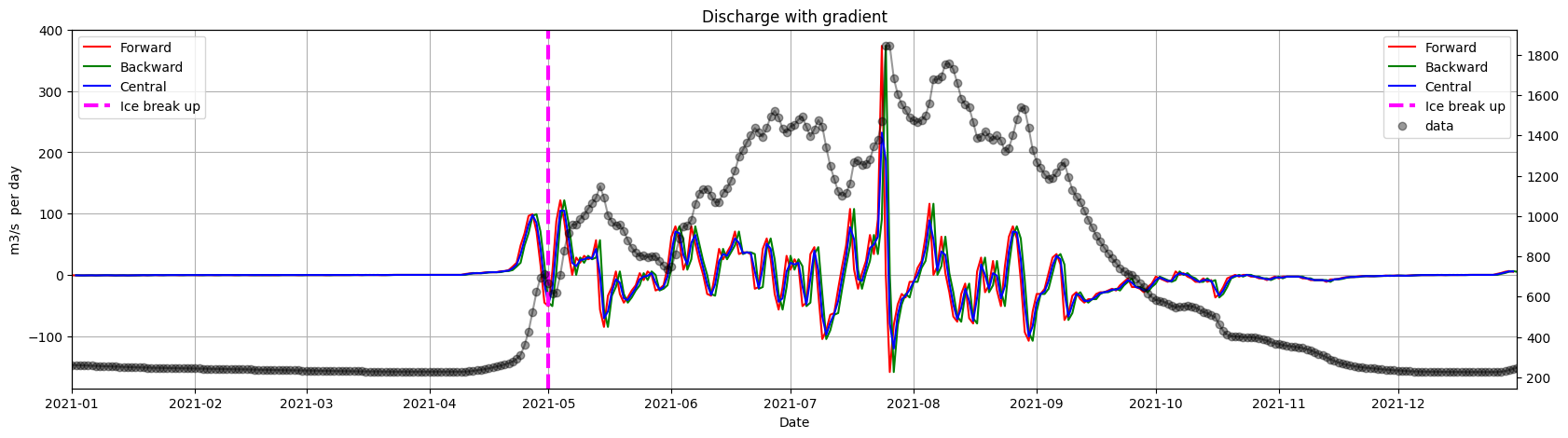
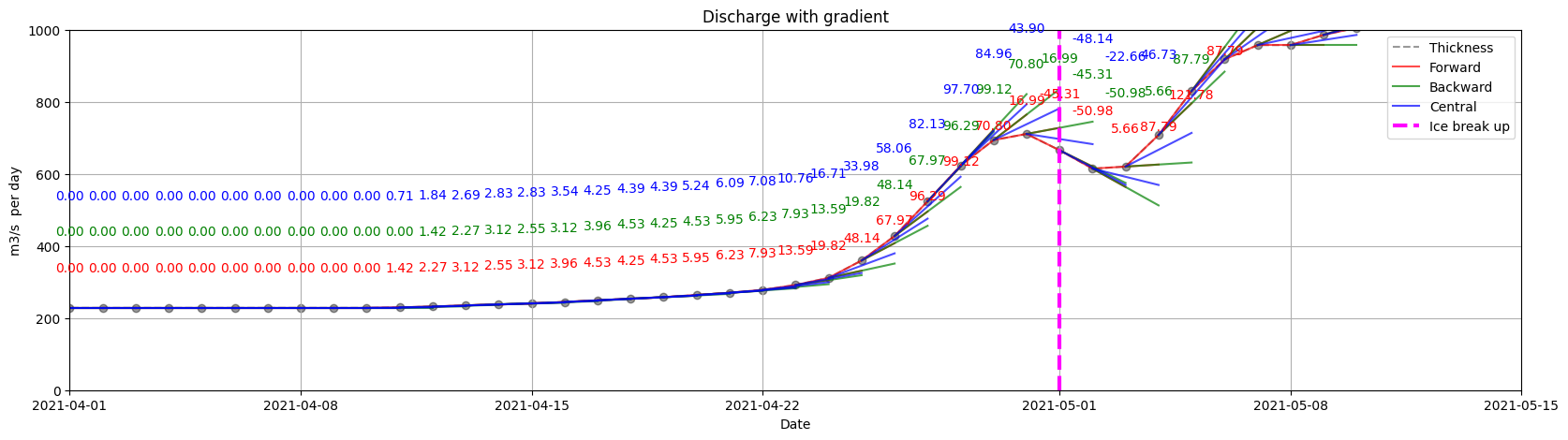
Discharge#
fix plotting function, so than when selecting an xlim, the function only compute the data in that range, right now it computes all the data and then restricts the plot which is slow
print(type(break_up_dates[break_up_dates.year == 2019].strftime('%m/%d')[0]))
Discharge=Data['Nenana: Mean Discharge [m3/s]']
Discharge=Discharge.dropna(inplace=False) # drop the missing values
result_2 = Discharge.groupby(Discharge.index.year,group_keys=True).apply(lambda x: ice.finite_differences(x))
result_2 = result_2.reset_index(level=0, drop=True)

ice.plot_gradients_and_timeseries(result_2,
                            Discharge,
                            2021,
                            Title='Discharge with gradient',
                            ylabel='m3/s  per day',
                            vline={'Ice break up': break_up_dates[break_up_dates.year == 2021].strftime('%m/%d')[0]})

ice.plot_gradients_and_timeseries(result_2,
                            Discharge,
                            2021,
                            plot_gradient_as_slope=True,
                            xlim=['04/01', '05/15'],
                            Title='Discharge with gradient',
                            ylabel='m3/s  per day',
                            ylim=[0, 1000],
                            annotation_offsets={'forward': 100, 'backward': 200, 'central': 300},
                            vline={'Ice break up': break_up_dates[break_up_dates.year == 2021].strftime('%m/%d')[0]})
#
<class 'str'>
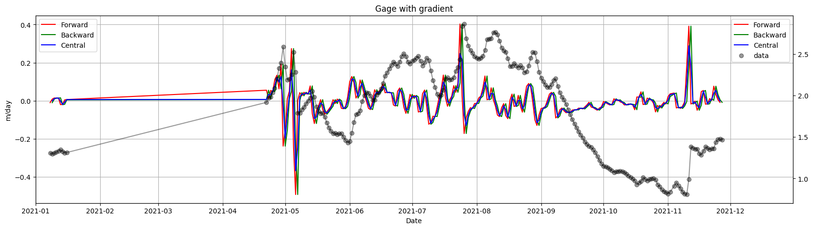
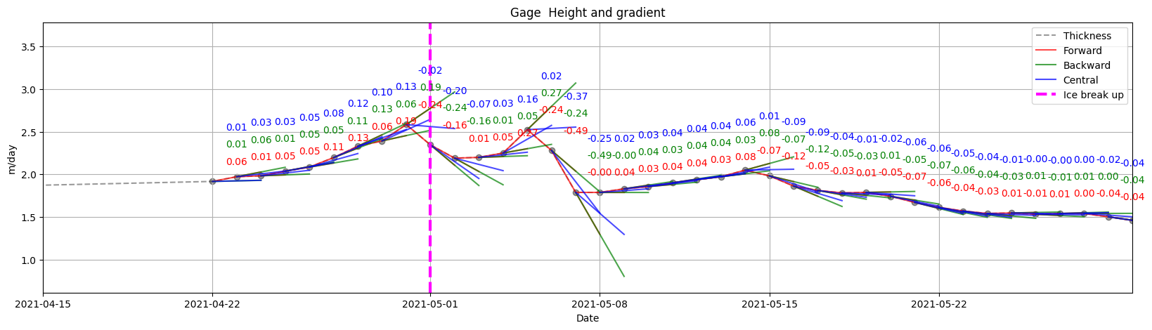
Gage Height#
Gage=Data['Nenana: Gage Height [m]']
Gage=Gage.dropna(inplace=False) # drop the missing values
result_3 = Gage.groupby(Gage.index.year,group_keys=True).apply(lambda x: ice.finite_differences(x))
result_3 = result_3.reset_index(level=0, drop=True)

ice.plot_gradients_and_timeseries(result_3,
                            Gage,
                            2021,
                            Title='Gage with gradient'
                            ,ylabel='m/day')

ice.plot_gradients_and_timeseries(result_3,
                            Gage,
                            2021,
                            plot_gradient_as_slope=True,
                            xlim=['04/15', '05/30'],
                            annotation_offsets={'forward': 0.2, 'backward': 0.4, 'central': 0.6},
                            ylabel='m/day',Title='Gage  Height and gradient',
                            vline={'Ice break up': break_up_dates[break_up_dates.year == 2021].strftime('%m/%d')[0]})