Week 1 Iceclassic Content and Plots#
Importing files and selecting the datasets that we will use#
import pandas as pd
from datetime import time ,datetime,timedelta
import pprint # for printing dictionaries
import matplotlib.pyplot as plt
from funciones import*


#Break up dates list
dates = pd.read_csv('../../data/List_break_up_dates.csv',names=['date_time'],header=None)
dates['date_time']=pd.to_datetime(dates['date_time'])


# External Variables
Data=pd.read_csv("../../data/Time_series_DATA.txt",skiprows=149,index_col=0,sep='\t')
Data.index = pd.to_datetime(Data.index, format="%Y-%m-%d")
# Data = Data[(Data.index.year >= 1917) & (Data.index.year < 2024)]
# selected_cols=['Regional: Air temperature [C]','Nenana: Rainfall [mm]','Nenana: Snowfall [mm]','Nenana: Mean Discharge [m3/s]','IceThickness [cm]']
# Data=Data[selected_cols]
Gage=pd.read_csv('../../data/raw_files/Nenana_Gage.txt',skiprows=24,sep='\t')
Gage['datetime'] = pd.to_datetime(Gage['datetime'])
Gage_mean= Gage.groupby(Gage['datetime'].dt.date)['1832_00065'].mean().reset_index()


Gage_mean.rename(columns={'datetime': 'date'}, inplace=True)
Gage_mean['Nenana: Gage Height [m]'] = Gage_mean['1832_00065'] * 0.3048
Gage_Height = Gage_mean[['date', 'Nenana: Gage Height [m]']]
Gage_Height.set_index('date', inplace=True)

df_merged = Data.merge(Gage_Height, left_index=True, right_index=True, how='left')

df_merged.to_csv('../../data/Time_series_DATA_Gage_Height.csv',sep='\t')
df_merged.index = pd.to_datetime(df_merged.index, format="%Y-%m-%d")
print(df_merged)

# explore_contents(df_merged)
Regional: Air temperature [C] Days since start of year \
1901-02-01 NaN NaN
1901-03-01 NaN NaN
1901-04-01 NaN NaN
1901-05-01 NaN NaN
1901-06-01 NaN NaN
... ... ...
2024-02-02 NaN NaN
2024-02-03 NaN NaN
2024-02-04 NaN NaN
2024-02-05 NaN NaN
2024-02-06 NaN NaN
Days until break up Nenana: Rainfall [mm] Nenana: Snowfall [mm] \
1901-02-01 NaN NaN NaN
1901-03-01 NaN NaN NaN
1901-04-01 NaN NaN NaN
1901-05-01 NaN NaN NaN
1901-06-01 NaN NaN NaN
... ... ... ...
2024-02-02 NaN NaN NaN
2024-02-03 NaN NaN NaN
2024-02-04 NaN NaN NaN
2024-02-05 NaN NaN NaN
2024-02-06 NaN NaN NaN
Nenana: Snow depth [mm] Nenana: Mean water temperature [C] \
1901-02-01 NaN NaN
1901-03-01 NaN NaN
1901-04-01 NaN NaN
1901-05-01 NaN NaN
1901-06-01 NaN NaN
... ... ...
2024-02-02 NaN NaN
2024-02-03 NaN NaN
2024-02-04 NaN NaN
2024-02-05 NaN NaN
2024-02-06 NaN NaN
Nenana: Mean Discharge [m3/s] Nenana: Air temperature [C] \
1901-02-01 NaN NaN
1901-03-01 NaN NaN
1901-04-01 NaN NaN
1901-05-01 NaN NaN
1901-06-01 NaN NaN
... ... ...
2024-02-02 221.1792 NaN
2024-02-03 221.1792 NaN
2024-02-04 220.8960 NaN
2024-02-05 220.8960 NaN
2024-02-06 2916.9600 NaN
Fairbanks: Average wind speed [m/s] ... \
1901-02-01 NaN ...
1901-03-01 NaN ...
1901-04-01 NaN ...
1901-05-01 NaN ...
1901-06-01 NaN ...
... ... ...
2024-02-02 NaN ...
2024-02-03 NaN ...
2024-02-04 NaN ...
2024-02-05 NaN ...
2024-02-06 NaN ...
Regional: Solar Surface Irradiance [W/m2] \
1901-02-01 NaN
1901-03-01 NaN
1901-04-01 NaN
1901-05-01 NaN
1901-06-01 NaN
... ...
2024-02-02 NaN
2024-02-03 NaN
2024-02-04 NaN
2024-02-05 NaN
2024-02-06 NaN
Regional: Cloud coverage [%] \
1901-02-01 62.675003
1901-03-01 63.737503
1901-04-01 56.087500
1901-05-01 68.212510
1901-06-01 76.225006
... ...
2024-02-02 NaN
2024-02-03 NaN
2024-02-04 NaN
2024-02-05 NaN
2024-02-06 NaN
Global: ENSO-Southern oscillation index Gulkana Temperature [C] \
1901-02-01 NaN NaN
1901-03-01 NaN NaN
1901-04-01 NaN NaN
1901-05-01 NaN NaN
1901-06-01 NaN NaN
... ... ...
2024-02-02 NaN NaN
2024-02-03 NaN NaN
2024-02-04 NaN NaN
2024-02-05 NaN NaN
2024-02-06 NaN NaN
Gulkana Precipitation [mm] \
1901-02-01 NaN
1901-03-01 NaN
1901-04-01 NaN
1901-05-01 NaN
1901-06-01 NaN
... ...
2024-02-02 NaN
2024-02-03 NaN
2024-02-04 NaN
2024-02-05 NaN
2024-02-06 NaN
Gulkana: Glacier-wide winter mass balance [m.w.e] \
1901-02-01 NaN
1901-03-01 NaN
1901-04-01 NaN
1901-05-01 NaN
1901-06-01 NaN
... ...
2024-02-02 NaN
2024-02-03 NaN
2024-02-04 NaN
2024-02-05 NaN
2024-02-06 NaN
Gulkana: Glacier-wide summer mass balance [m.w.e] \
1901-02-01 NaN
1901-03-01 NaN
1901-04-01 NaN
1901-05-01 NaN
1901-06-01 NaN
... ...
2024-02-02 NaN
2024-02-03 NaN
2024-02-04 NaN
2024-02-05 NaN
2024-02-06 NaN
Global: Pacific decadal oscillation index \
1901-02-01 NaN
1901-03-01 NaN
1901-04-01 NaN
1901-05-01 NaN
1901-06-01 NaN
... ...
2024-02-02 NaN
2024-02-03 NaN
2024-02-04 NaN
2024-02-05 NaN
2024-02-06 NaN
Global: Artic oscillation index Nenana: Gage Height [m]
1901-02-01 NaN NaN
1901-03-01 NaN NaN
1901-04-01 NaN NaN
1901-05-01 NaN NaN
1901-06-01 NaN NaN
... ... ...
2024-02-02 NaN NaN
2024-02-03 NaN NaN
2024-02-04 NaN NaN
2024-02-05 NaN NaN
2024-02-06 NaN NaN
[39309 rows x 25 columns]
1. Use dictionaries to store dataset metadata and information about break-up years#
We use groupby-apply-tranform in variables from Data(df with all the data) to collapse a year of data to a single value per year, then re-index to align.
# creating a dictionary for every break up date, then creating a dictionary with the dictionaries
dates = pd.read_csv('../../data/List_break_up_dates.csv',names=['date_time'],header=None)
dates['date_time']=pd.to_datetime(dates['date_time'])


#=========================================================================================#
#  keys related to break_up dates
#=========================================================================================#
dates['year']=dates['date_time'].dt.year
dates['month']=dates['date_time'].dt.strftime('%B')
dates['day']=dates['date_time'].dt.day
dates['day_of_year']=dates['date_time'].dt.dayofyear

dates.index=dates['year']

dates['days_since_01_apr']=dates['date_time'].apply(lambda dt : (dt-pd.Timestamp(year=dt.year,month=4,day=1)).days)
dates['time']=dates['date_time'].dt.time
dates['hour']=dates['date_time'].dt.hour
dates['minute']=dates['date_time'].dt.minute

dates['decimal_time']=round(dates['date_time'].dt.time.apply(lambda t: decimal_time(t,direction='to_decimal')),4)
dates['decimal_day_of_year']=round(dates['time'].apply(lambda t: decimal_day(t,direction='to_decimal'))+dates['day_of_year'],8)
# decimal day
# decimal year, etc


#=========================================================================================#
#  keys related to ice_thickness
#=========================================================================================#
Ice=Data['IceThickness [cm]'].dropna()  # to make the following lines cleaner
dates['max_ice_thickness'] =Ice.groupby(Ice.index.year).max().reindex(dates.index,method=None)
dates['day_of_max_ice_thickness']=Ice.groupby(Ice.index.year).idxmax().reindex(dates.index,method=None)
dates['last_ice_measurement']=Ice.groupby(Ice.index.year).last().reindex(dates.index,method=None)
dates['day_of_last_ice_measurement']=Ice.groupby(Ice.index.year).apply(lambda x: x.index[-1]).reindex(dates.index,method=None)

dates['n_days_last_measured_ice_&_break_up']=dates.apply( lambda row: (row['day_of_last_ice_measurement']-row['date_time']).days if pd.notna(row['day_of_last_ice_measurement']) and pd.notna(row['date_time']) else None,axis=1)


dates['final_melting_gradient[cm/day]']=Ice.groupby(Ice.index.year).apply(lambda x: (x.iloc[-2]-x.iloc[-1])/(x.index[-2]-x.index[-1]).days).round(3).reindex(dates.index,method=None)
# if we define that break up happens wiht ice thickness equal to zero, the final melting gradient would be computed diffentle, but not always the break-up happens when the thickness is zero.
dates['melting_gradient_if_breakup_happens_at_zero-thickness[cm/day]']=round(dates['last_ice_measurement']/dates['n_days_last_measured_ice_&_break_up'],3)
#=========================================================================================#
#  keys related to temperature
#=========================================================================================#
Temp=Data['Regional: Air temperature [C]'].dropna()
dates['days_over_minus_2'] = Temp.groupby(Temp.index.year).apply(lambda x: (x > -2).sum()).astype(int).reindex(dates.index,method=None) # assumes that the number of day over 1 since the start of ice formation to jan 01 is zero
dates['cumsum_over_2_temp']= Temp.groupby(Temp.index.year).apply(lambda x: x.clip(lower=0).where(x > 2).sum()).round(3).reindex(dates.index,method=None)
dates['avg_temp']=Temp.groupby(Temp.index.year).mean().round(2)
# min tem, max temp, min tem in jan, etc

#=========================================================================================#
#  converting df to dict of dict and list of dict
#=========================================================================================#

# print('Printing Dataframe\n=====================')
# print(dates)

dict_of_dict=dates.to_dict(orient='index')
#print('Printing dict of dict\n=====================')
#pprint.pprint(dict_of_dict,sort_dicts=False) # to avoid PrettyPrint printing the keys alphabetically


# list_of_dict=dates.to_dict(orient='records')
# print('Printing list of dict\n=====================')
# pprint.pprint(list_of_dict,sort_dict-False)


#=========================================================================================#
#  accessing element of dict_of_dict
#=========================================================================================#
# because we assigned the year to each dict we can simply pass the year to get the data related to the break up of that year
pprint.pprint(dict_of_dict[2015],sort_dicts=False)
{'date_time': Timestamp('2015-04-24 14:25:00'),
 'year': 2015,
 'month': 'April',
 'day': 24,
 'day_of_year': 114,
 'days_since_01_apr': 23,
 'time': datetime.time(14, 25),
 'hour': 14,
 'minute': 25,
 'decimal_time': 14.4167,
 'decimal_day_of_year': 114.60069444,
 'max_ice_thickness': 97.79,
 'day_of_max_ice_thickness': Timestamp('2015-03-05 00:00:00'),
 'last_ice_measurement': 85.09,
 'day_of_last_ice_measurement': Timestamp('2015-04-06 00:00:00'),
 'n_days_last_measured_ice_&_break_up': -19.0,
 'final_melting_gradient[cm/day]': -1.27,
 'melting_gradient_if_breakup_happens_at_zero-thickness[cm/day]': -4.478,
 'days_over_minus_2': 219.0,
 'cumsum_over_2_temp': 1754.84,
 'avg_temp': -0.77}
2. Datasets are stored as a dictionary of dictionaries:#
variable_summary={}

n_total=len(Data.index.year.unique())
print(n_total)

for column in Data.columns:
    first_obs=Data.index.year.min()
    last_obs=Data.index.year.max()
    avg_n_obs_yearly=Data[column].groupby(Data.index.year).count().mean().round(2)
    historic_max=Data[column].max().round(2)
    yearly_avg=Data[column].mean().round(2)
    n_years=Data[Data[column].notna()].index.year.unique()
    n_year_percent=round((len(n_years)/n_total*100),2)
    variable_summary[column]={
        'year_start':first_obs,
        'year_end':last_obs,
        'avg_n_yearly': avg_n_obs_yearly,
        'historic_max': historic_max,
        'yearly_avg': yearly_avg,
        'years_present (%)':n_year_percent,
        'years_present':n_years}


pprint.pprint(variable_summary['Regional: Air temperature [C]'],sort_dicts=False)
124
{'year_start': 1901,
 'year_end': 2024,
 'avg_n_yearly': 310.99,
 'historic_max': 23.23,
 'yearly_avg': -2.61,
 'years_present (%)': 85.48,
 'years_present': Index([1917, 1918, 1919, 1920, 1921, 1922, 1923, 1924, 1925, 1926,
       ...
       2013, 2014, 2015, 2016, 2017, 2018, 2019, 2020, 2021, 2022],
      dtype='int32', length=106)}
To get more info we can always use the function
explore_contentsfrom the iceclassic package, more ways to visualize the contents can be seen in the book sectionLoading_&_Exploring_Data.ipynb, like the interactive plots and the timeseries plots/distribution of each variable/column
3. Time Series Plots#
3.1/3.2/3.3 Plotting, labels and highlighting years#
We will use a slightly updated version from the function plot_contents from the iceclassic package, the updated version can be found in /funciones.py, and has not been
committed/uploaded to its individual repo nor released to PyPi
\
More examples on how to use the function can be found in the book in the section Seasonality(groupby-transform-apply).ipynb
# we reload df cuz we need some column that we dropped at the beginning
Data=pd.read_csv("../../data/Time_series_DATA.txt",skiprows=149,index_col=0,sep='\t')
Data.index = pd.to_datetime(Data.index, format="%Y-%m-%d")
Data = Data[(Data.index.year >= 1917) & (Data.index.year < 2024)]
Data.info()

plot_contents(df_merged,
              columns_to_plot=['Regional: Air temperature [C]','Nenana: Mean Discharge [m3/s]','Nenana: Gage Height [m]'],     # what columns to plot, default all
              col_cmap=['grey'],                                     # list of colors for each column, default is sequential cmap, but list of colors can be passed as well
              scatter_alpha=0.2,                                     # we can 'mute' the scatter points if we choose lapha=0, then the col_map is irrelevant, cuz the scatter markers are no being plotted
              plot_mean_std=False,                                   # we 'mute' the baseline across all years, similar here, if it were 'True' the color would have been grey'
              multiyear=[2019,1998,2013],                            # we select which years to highlight
              years_line_width=2,                                    # change the iwth of line if necessary
              plot_break_up_dates=True,
              xaxis='Days until break up')                              # plotting break_up_dates makers with annotations, default =False
<class 'pandas.core.frame.DataFrame'>
DatetimeIndex: 39081 entries, 1917-01-01 to 2023-12-31
Data columns (total 24 columns):
 #   Column                                             Non-Null Count  Dtype
---  ------                                             --------------  -----
 0   Regional: Air temperature [C]                      38563 non-null  float64
 1   Days since start of year                           38563 non-null  float64
 2   Days until break up                                38563 non-null  float64
 3   Nenana: Rainfall [mm]                              29516 non-null  float64
 4   Nenana: Snowfall [mm]                              19945 non-null  float64
 5   Nenana: Snow depth [mm]                            15984 non-null  float64
 6   Nenana: Mean water temperature [C]                 2418 non-null   float64
 7   Nenana: Mean Discharge [m3/s]                      22525 non-null  float64
 8   Nenana: Air temperature [C]                        31146 non-null  float64
 9   Fairbanks: Average wind speed [m/s]                9797 non-null   float64
 10  Fairbanks: Rainfall [mm]                           29586 non-null  float64
 11  Fairbanks: Snowfall [mm]                           29586 non-null  float64
 12  Fairbanks: Snow depth [mm]                         29555 non-null  float64
 13  Fairbanks: Air Temperature [C]                     29587 non-null  float64
 14  IceThickness [cm]                                  461 non-null    float64
 15  Regional: Solar Surface Irradiance [W/m2]          86 non-null     float64
 16  Regional: Cloud coverage [%]                       1272 non-null   float64
 17  Global: ENSO-Southern oscillation index            876 non-null    float64
 18  Gulkana Temperature [C]                            19146 non-null  float64
 19  Gulkana Precipitation [mm]                         18546 non-null  float64
 20  Gulkana: Glacier-wide winter mass balance [m.w.e]  58 non-null     float64
 21  Gulkana: Glacier-wide summer mass balance [m.w.e]  58 non-null     float64
 22  Global: Pacific decadal oscillation index          1284 non-null   float64
 23  Global: Artic oscillation index                    888 non-null    float64
dtypes: float64(24)
memory usage: 7.5 MB
No Nenana: Gage Height [m] data available for year 1998
fix, move scatter point to the front of plot, add arrows between the label and the point.
the argument xlim can be passe to restrict the xaxis
from funciones import*
# we reload df cuz we need days to breal up and days of year colums
Data=pd.read_csv("../../data/Time_series_DATA.txt",skiprows=149,index_col=0,sep='\t')
Data.index = pd.to_datetime(Data.index, format="%Y-%m-%d")
Data = Data[(Data.index.year >= 1917) & (Data.index.year < 2024)]
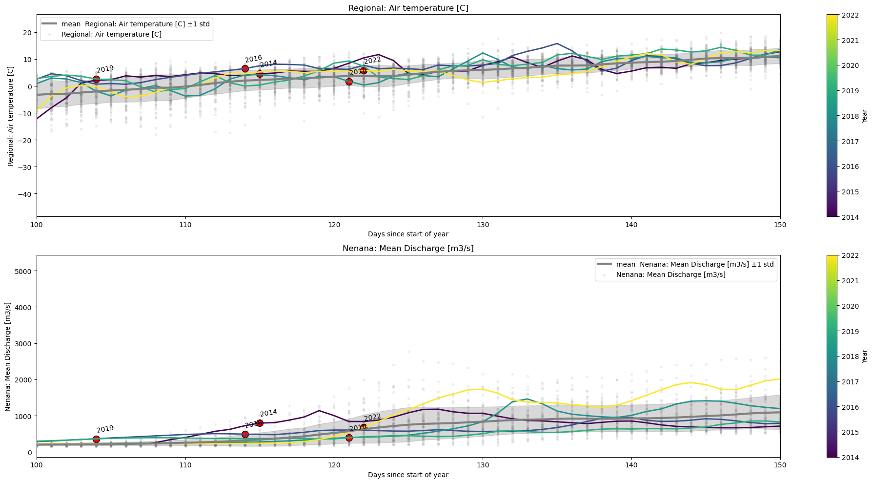
plot_contents(df_merged,
columns_to_plot=['Regional: Air temperature [C]','Nenana: Mean Discharge [m3/s]'], # what column to plot, default all
col_cmap=['grey'], # list of colors for each column, default is sequential cmap
scatter_alpha=0.1, # we 'mute' the scatter points
plot_mean_std=True, # now we plot the baseline across all years
multiyear=[2014,2016,2018,2019,2022], # we select which years to choose
plot_break_up_dates=True, # plotting break_up_dates scatter default =False
years_line_width=2, # line with a litlte bit narrower than dafault=4
xlim=[100,150]) # xlimits
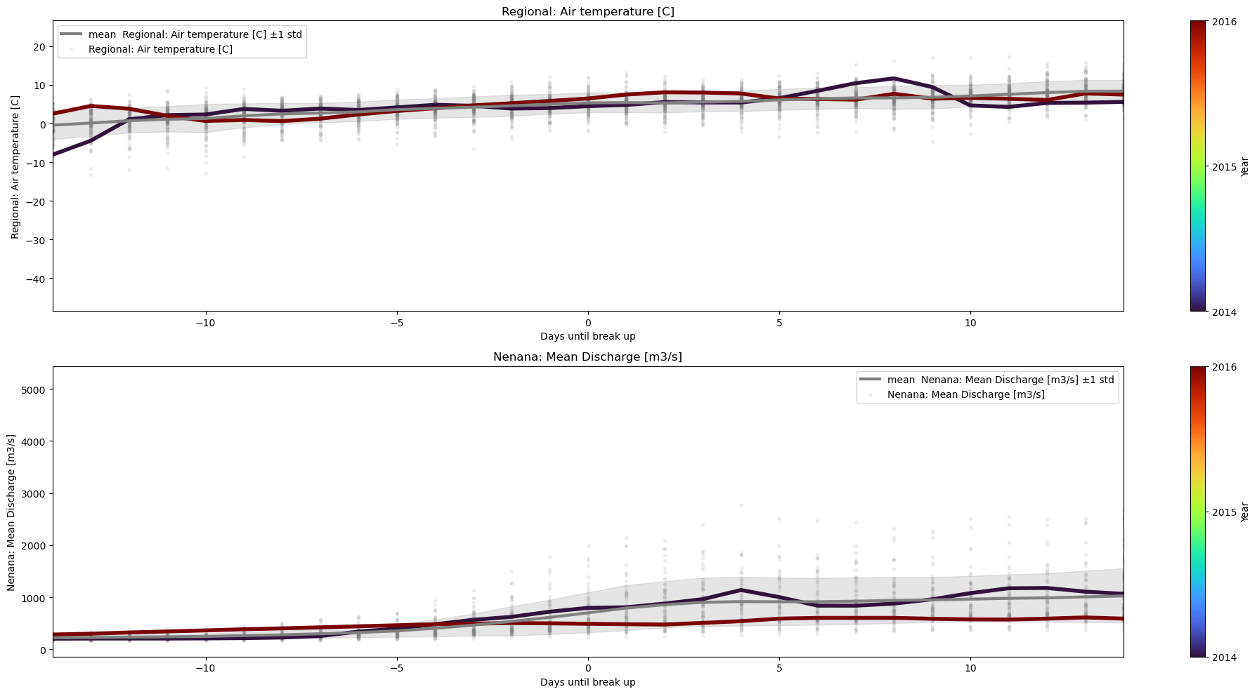
3.4 Normalizing x-axis#
The easiest way to normalize xaxis is by choosing xaxis=’Days until break up’ ( which is a column in Data).
With this axis, there is no need to put annotations with the year, because we know that data is normalized such that the breakup happens at xaxis=0.
plot_contents(Data,
              xaxis='Days until break up',
              columns_to_plot=['Regional: Air temperature [C]','Nenana: Mean Discharge [m3/s]'],    # what column to plot, default all
              col_cmap=['grey'],                                    # list of colors for each column, default is sequential cmap
              std_alpha=0.2,                                        # alpha for the fill
              plot_mean_std=True,                                   # if we put true the baseline plus scatter are plotted
              multiyear=[2014,2016],                                # we select which years to choose
              plot_break_up_dates=True,                             # plotting break_up_dates scatter default
              xlim=[-14,14],
              years_cmap='turbo')                                   # we can pass other cmaps for the colorbar
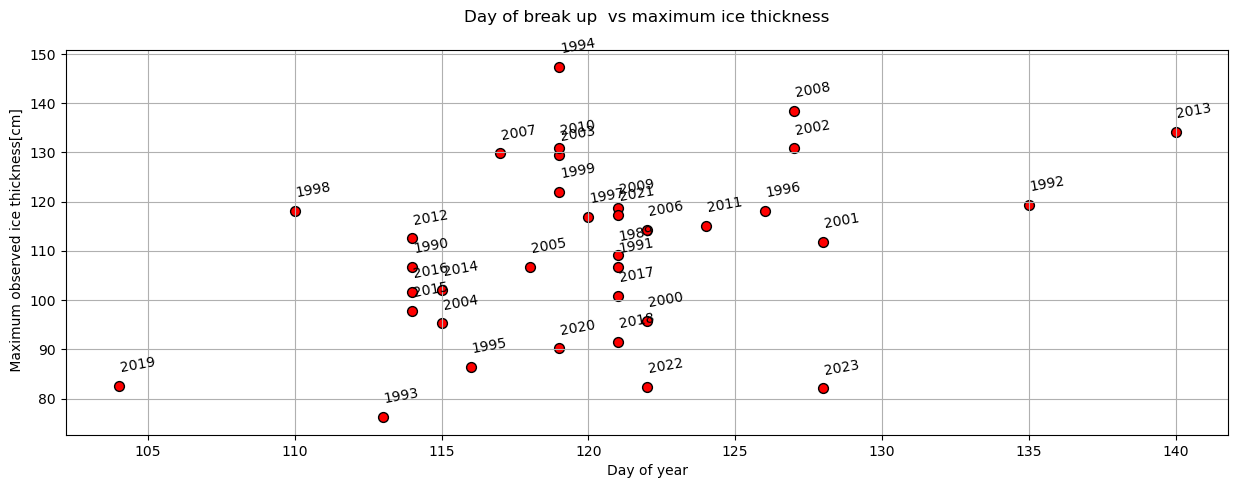
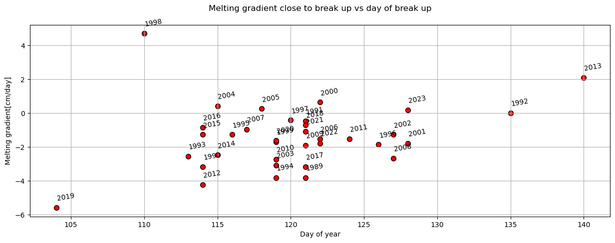
4. Scatter Plots#
Because the df/dict is already aligned, we can easily access and plot stuff.
We can use any of the column of dates as either x or y vectors.
dates.info()
plot_scatter(dates,'day_of_year','max_ice_thickness',x_label='Day of year',y_label=' Maximum observed ice thickness[cm]',title='Day of break up vs maximum ice thickness')
plot_scatter(dates,'day_of_year','final_melting_gradient[cm/day]',x_label='Day of year',y_label='Melting gradient[cm/day]',title='Melting gradient close to break up vs day of break up')
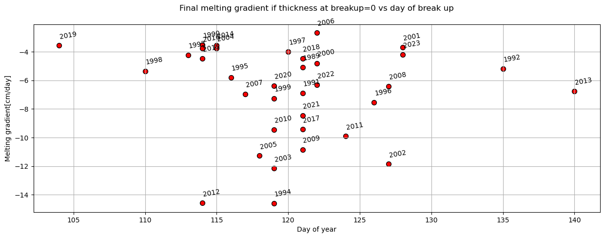
plot_scatter(dates,'day_of_year','melting_gradient_if_breakup_happens_at_zero-thickness[cm/day]',x_label='Day of year',y_label='Melting gradient[cm/day]',title='Final melting gradient if thickness at breakup=0 vs day of break up')
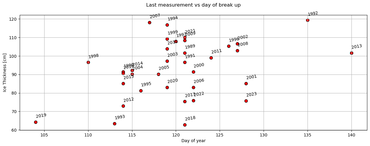
plot_scatter(dates,'day_of_year','last_ice_measurement',x_label='Day of year',y_label='Ice Thickness [cm]',title='Last measurement vs day of break up')
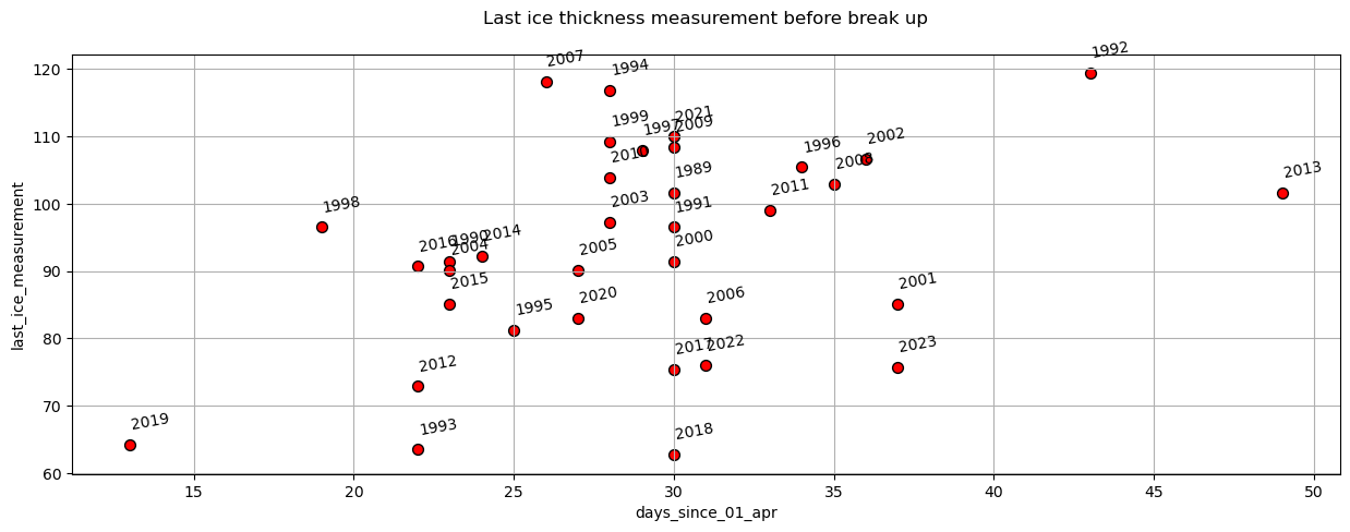
plot_scatter(dates,'days_since_01_apr','last_ice_measurement',title='Last ice thickness measurement before break up')
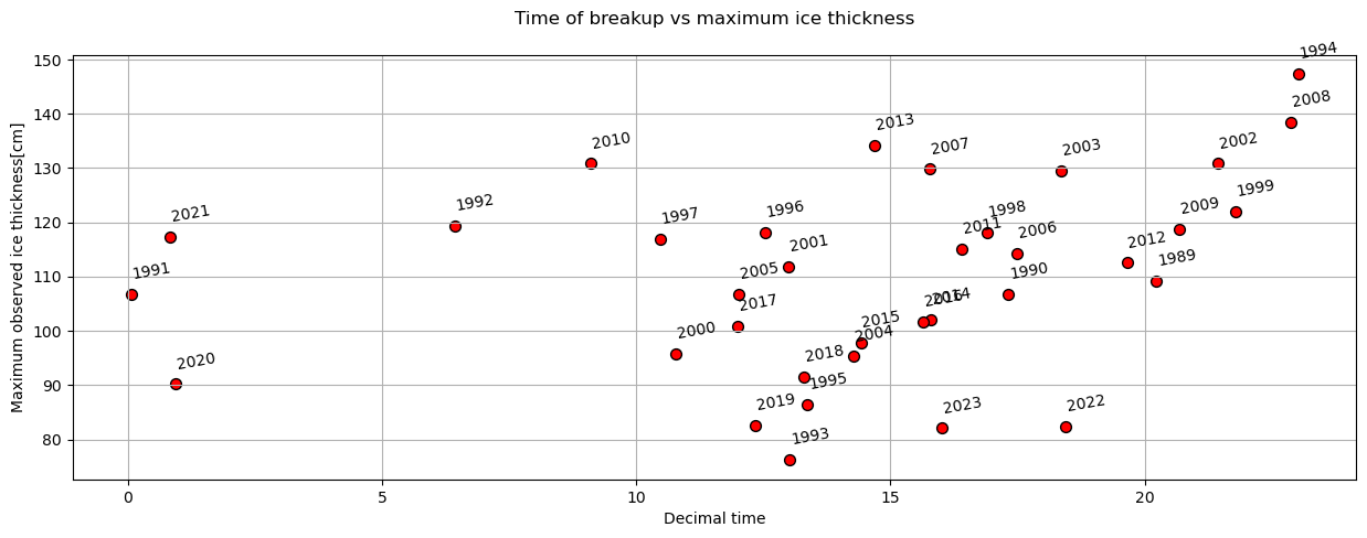
plot_scatter(dates,'decimal_time','max_ice_thickness',x_label='Decimal time',y_label='Maximum observed ice thickness[cm]',title='Time of breakup vs maximum ice thickness')
<class 'pandas.core.frame.DataFrame'>
Index: 107 entries, 1917 to 2023
Data columns (total 21 columns):
 #   Column                                                         Non-Null Count  Dtype
---  ------                                                         --------------  -----
 0   date_time                                                      107 non-null    datetime64[ns]
 1   year                                                           107 non-null    int32
 2   month                                                          107 non-null    object
 3   day                                                            107 non-null    int32
 4   day_of_year                                                    107 non-null    int32
 5   days_since_01_apr                                              107 non-null    int64
 6   time                                                           107 non-null    object
 7   hour                                                           107 non-null    int32
 8   minute                                                         107 non-null    int32
 9   decimal_time                                                   107 non-null    float64
 10  decimal_day_of_year                                            107 non-null    float64
 11  max_ice_thickness                                              35 non-null     float64
 12  day_of_max_ice_thickness                                       35 non-null     datetime64[ns]
 13  last_ice_measurement                                           35 non-null     float64
 14  day_of_last_ice_measurement                                    35 non-null     datetime64[ns]
 15  n_days_last_measured_ice_&_break_up                            35 non-null     float64
 16  final_melting_gradient[cm/day]                                 35 non-null     float64
 17  melting_gradient_if_breakup_happens_at_zero-thickness[cm/day]  35 non-null     float64
 18  days_over_minus_2                                              106 non-null    float64
 19  cumsum_over_2_temp                                             106 non-null    float64
 20  avg_temp                                                       106 non-null    float64
dtypes: datetime64[ns](3), float64(10), int32(5), int64(1), object(2)
memory usage: 19.0+ KB
Other plots#
Examples of other plots that we can make withe de function that we have.
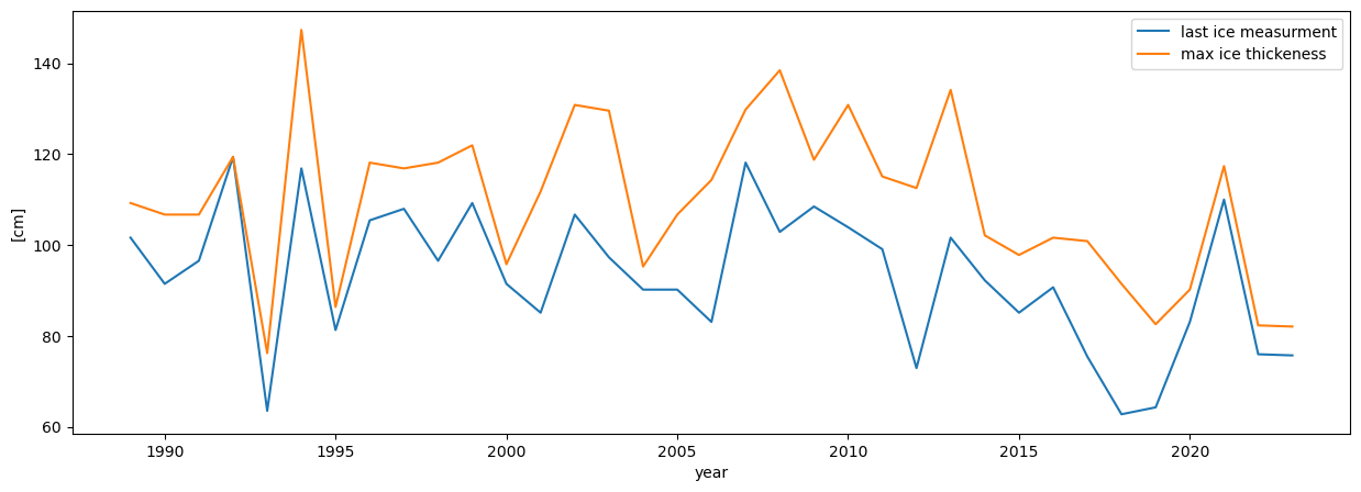
plt.figure(figsize=(15,5))
plt.plot(dates['last_ice_measurement'],label='last ice measurment')
plt.plot(dates['max_ice_thickness'],label='max ice thickeness')
plt.ylabel('[cm]')
plt.xlabel('year')
plt.legend()
plt.show()
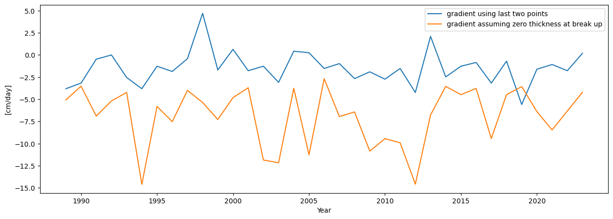
plt.figure(figsize=(15,5))
plt.plot(dates['final_melting_gradient[cm/day]'],label='gradient using last two points')
plt.plot(dates['melting_gradient_if_breakup_happens_at_zero-thickness[cm/day]'],label='gradient assuming zero thickness at break up')
plt.ylabel('[cm/day]')
plt.xlabel('Year')
plt.legend()
<matplotlib.legend.Legend at 0x1bb8323de10>
Other Scater/TimeSeries plots#
For scatter plot that use more than one value per year per variable, revert to using plot_contents, as we pass any column to use as xaxis.
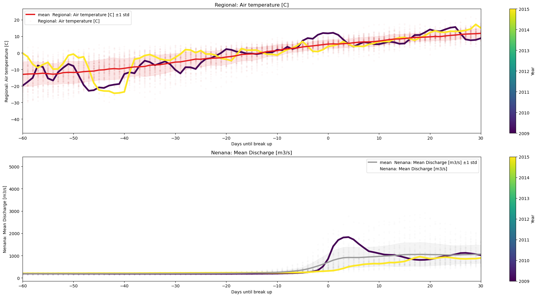
selected_years = [2009,2015]
plot_contents(Data,
              multiyear=selected_years,
              columns_to_plot=['Regional: Air temperature [C]','Nenana: Mean Discharge [m3/s]'],
              xaxis='Days until break up',
              xlim=[-60,30],
              plot_mean_std='true',
              scatter_alpha=.02,
              std_alpha=.1)
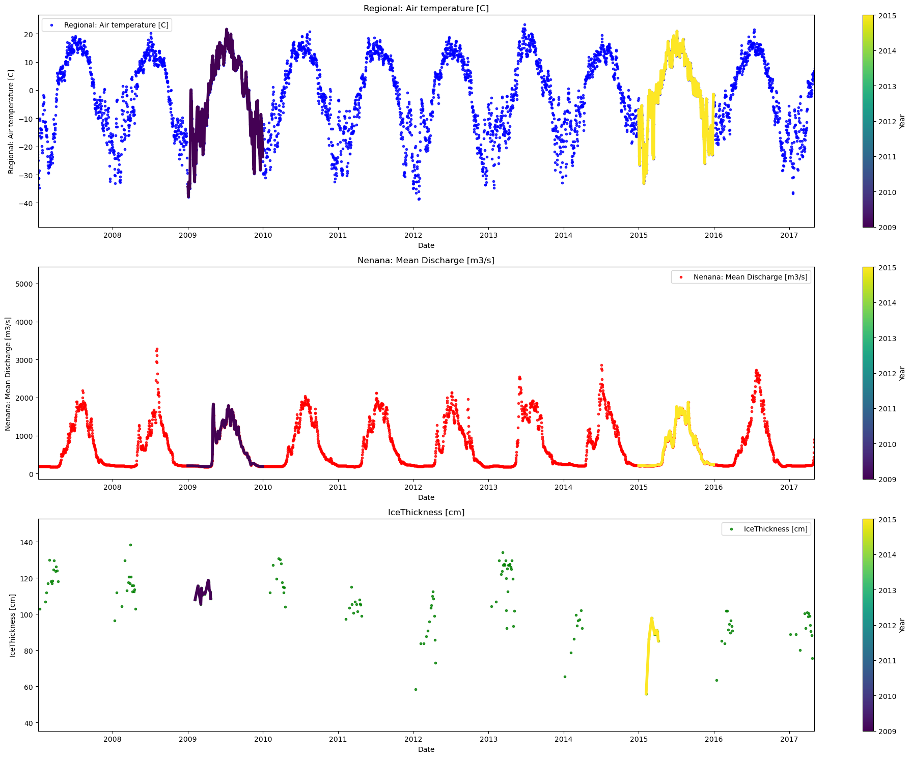
plot_contents(Data,
              multiyear=selected_years,
              columns_to_plot=['Regional: Air temperature [C]','Nenana: Mean Discharge [m3/s]','IceThickness [cm]'],
              xaxis='index',
              scatter_alpha=0.8,
              col_cmap=['blue','red','green'],
              xlim=['2007/01/04','2017/05/03'])
plot_contents(Data,
              columns_to_plot=['Regional: Air temperature [C]','Nenana: Mean Discharge [m3/s]','IceThickness [cm]'],
              plot_together=True,
              plot_mean_std='only',
              k=1,normalize='z-score',
              xaxis='Days until break up',col_cmap=['blue','red','green'])
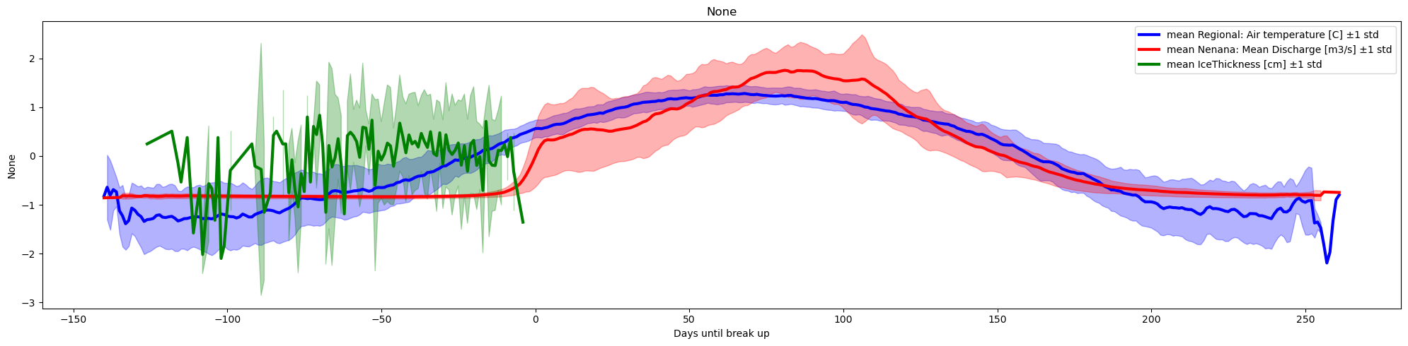
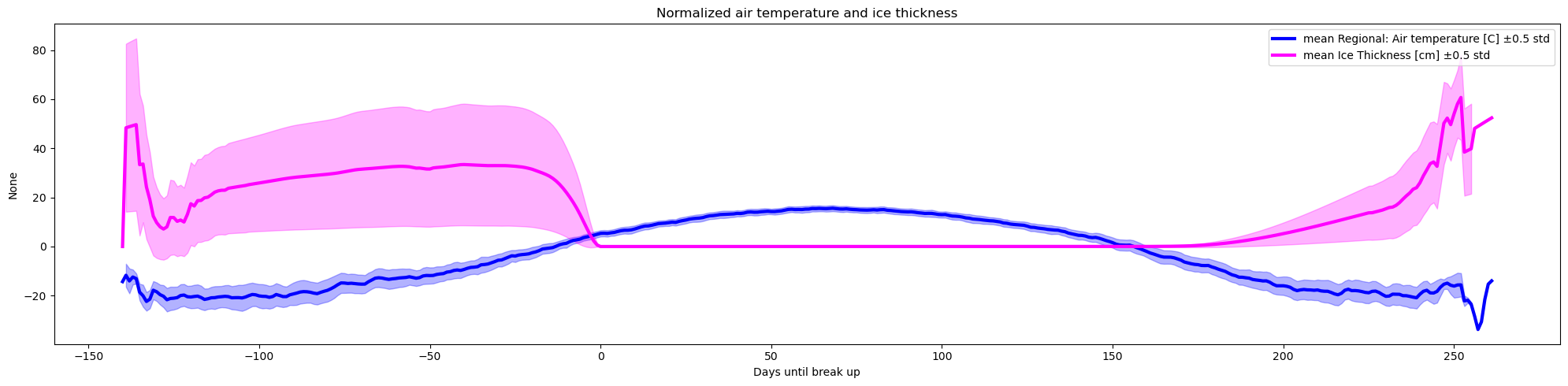
The IceThickness [cm] observations are relatively sparse ( ~10 per year), and are measured at different dates each year, therefore the plot considering the mean and std associated with the aggregated data (for each date) is not an accurate representation. We can fix this issue by interpolating the ice thickness (we assume ice start to grow on oct-15)
date = pd.Timestamp('2024-10-15')
oct_15 = date.dayofyear
Data.loc[(Data.index.dayofyear == oct_15), 'IceThickness [cm]'] = 0
Data.loc[(Data['Days until break up'] == 0), 'IceThickness [cm]'] = 0
ICE_pchip=Data['IceThickness [cm]'].interpolate(method='pchip')
ICE_pchip = ICE_pchip.clip(lower=0)

df_merged['Ice Thickness [cm]']=ICE_pchip
lets visually check the interpolation.
# plt.figure(figsize=(15,5))
# plt.scatter(Data.index,Data['IceThickness [cm]'],label='Original data',color='purple')
# plt.plot(Data.index,Data['Interpolated_IceThickness [cm]'],label='Interpolated data',color='orange')
# plt.xlim(pd.to_datetime(['1987/01/01','2024/01/01']))
plot_contents(df_merged,
              columns_to_plot=['Regional: Air temperature [C]','Ice Thickness [cm]'],
              plot_together=True,
              plot_mean_std='only',
              k=0.5,
              xaxis='Days until break up',col_cmap=['blue','magenta'],
              Title='Normalized air temperature and ice thickness')
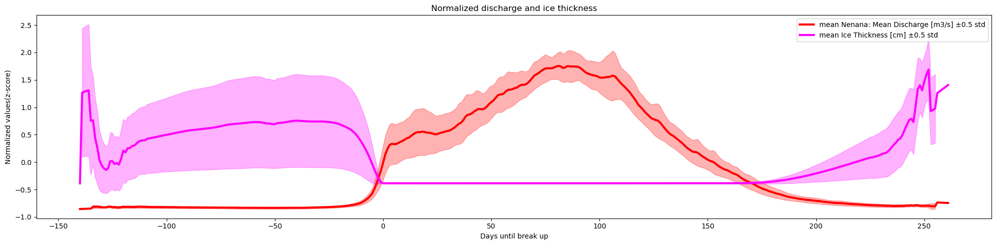
plot_contents(df_merged,
              columns_to_plot=['Nenana: Mean Discharge [m3/s]','Ice Thickness [cm]'],
              plot_together=True,
              plot_mean_std='only',
              k=0.5,normalize='z-score',
              xaxis='Days until break up',col_cmap=['red','magenta','magenta'],
              Title='Normalized discharge and ice thickness',
              y_label='Normalized values(z-score)')
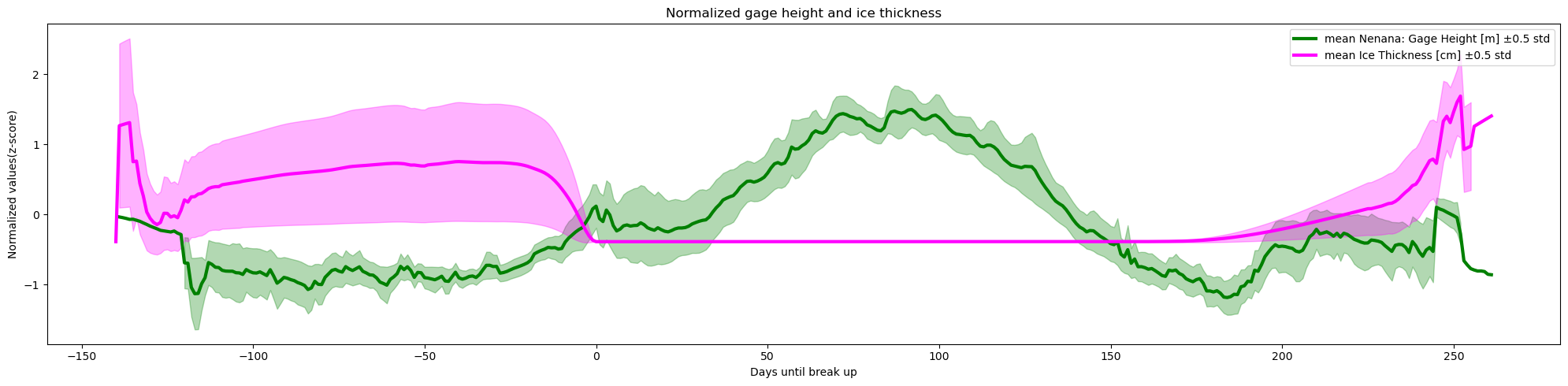
plot_contents(df_merged,
              columns_to_plot=['Nenana: Gage Height [m]', 'Ice Thickness [cm]'],
              plot_together=True,
              plot_mean_std='only',
              k=0.5,normalize='z-score',
              xaxis='Days until break up',col_cmap=['green','magenta'],
              Title='Normalized gage height and ice thickness',
              y_label='Normalized values(z-score)')
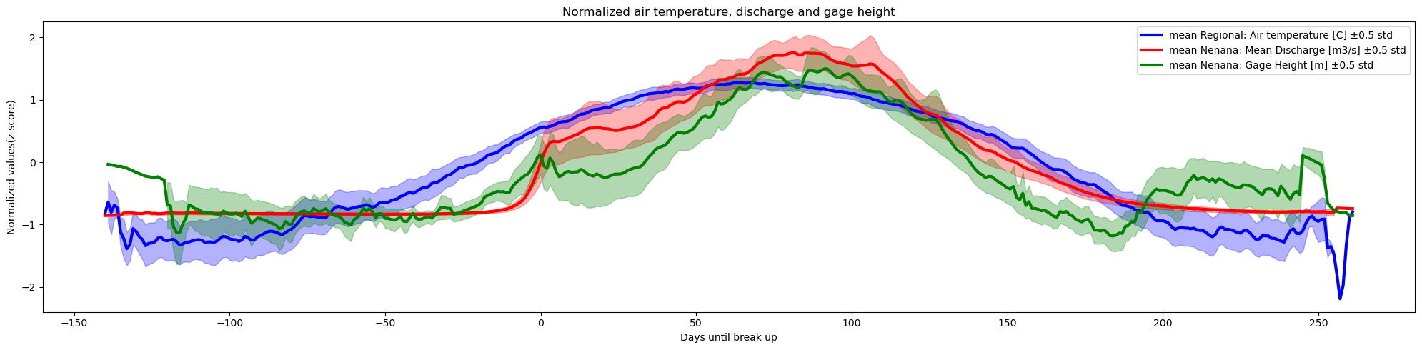
plot_contents(df_merged,
              columns_to_plot=['Regional: Air temperature [C]','Nenana: Mean Discharge [m3/s]','Nenana: Gage Height [m]'],
              plot_together=True,
              plot_mean_std='only',
              k=0.5,normalize='z-score',
              xaxis='Days until break up',col_cmap=['blue','red','green'],
              Title='Normalized air temperature, discharge and gage height',
              y_label='Normalized values(z-score)')
# # we reload df cuz we need some column that we dropped at the beginning
# Data=pd.read_csv("../../data/Time_series_DATA.txt",skiprows=149,index_col=0,sep='\t')
# Data.index = pd.to_datetime(Data.index, format="%Y-%m-%d")
# Data = Data[(Data.index.year >= 1917) & (Data.index.year < 2024)]
# Data.info()
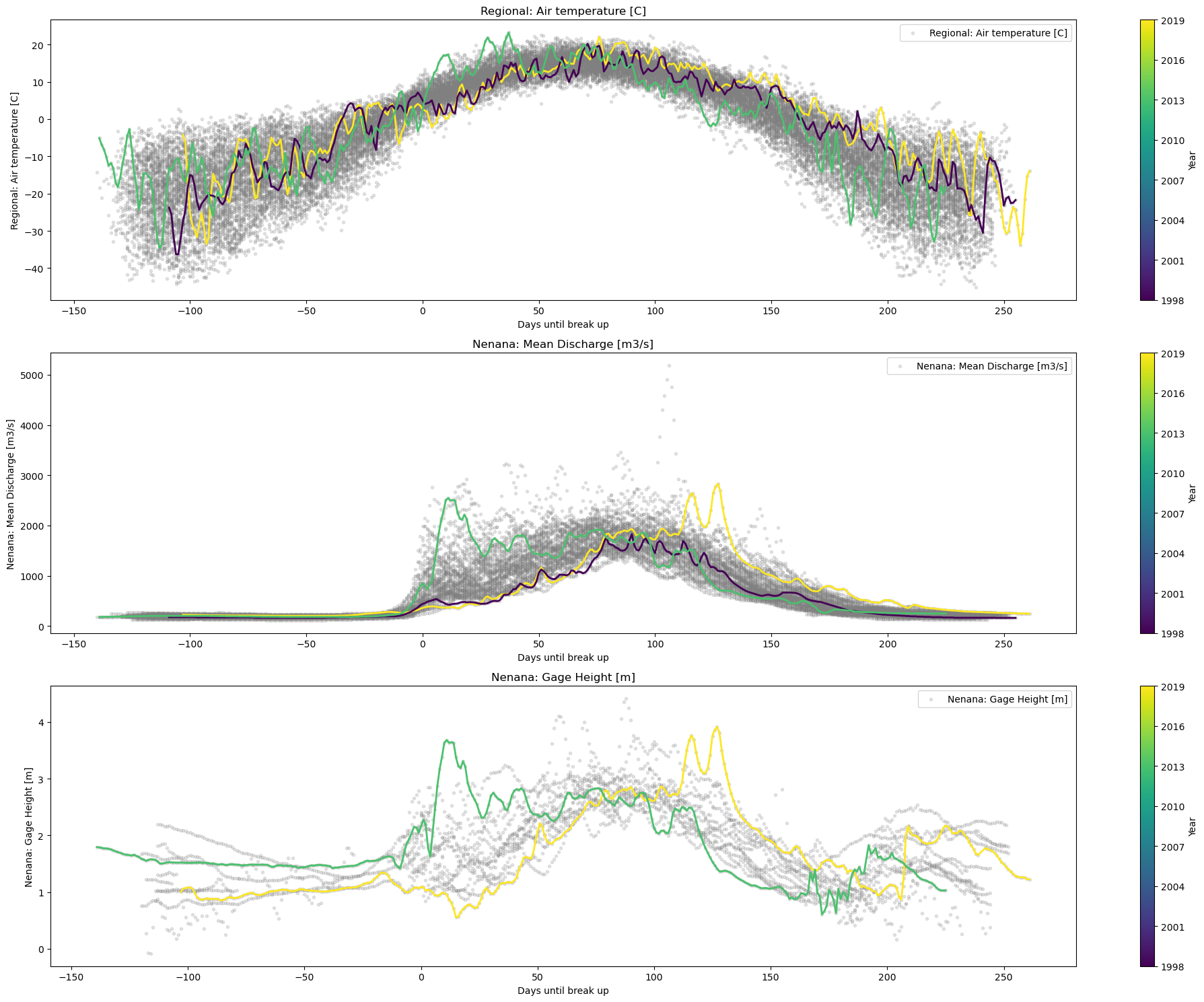
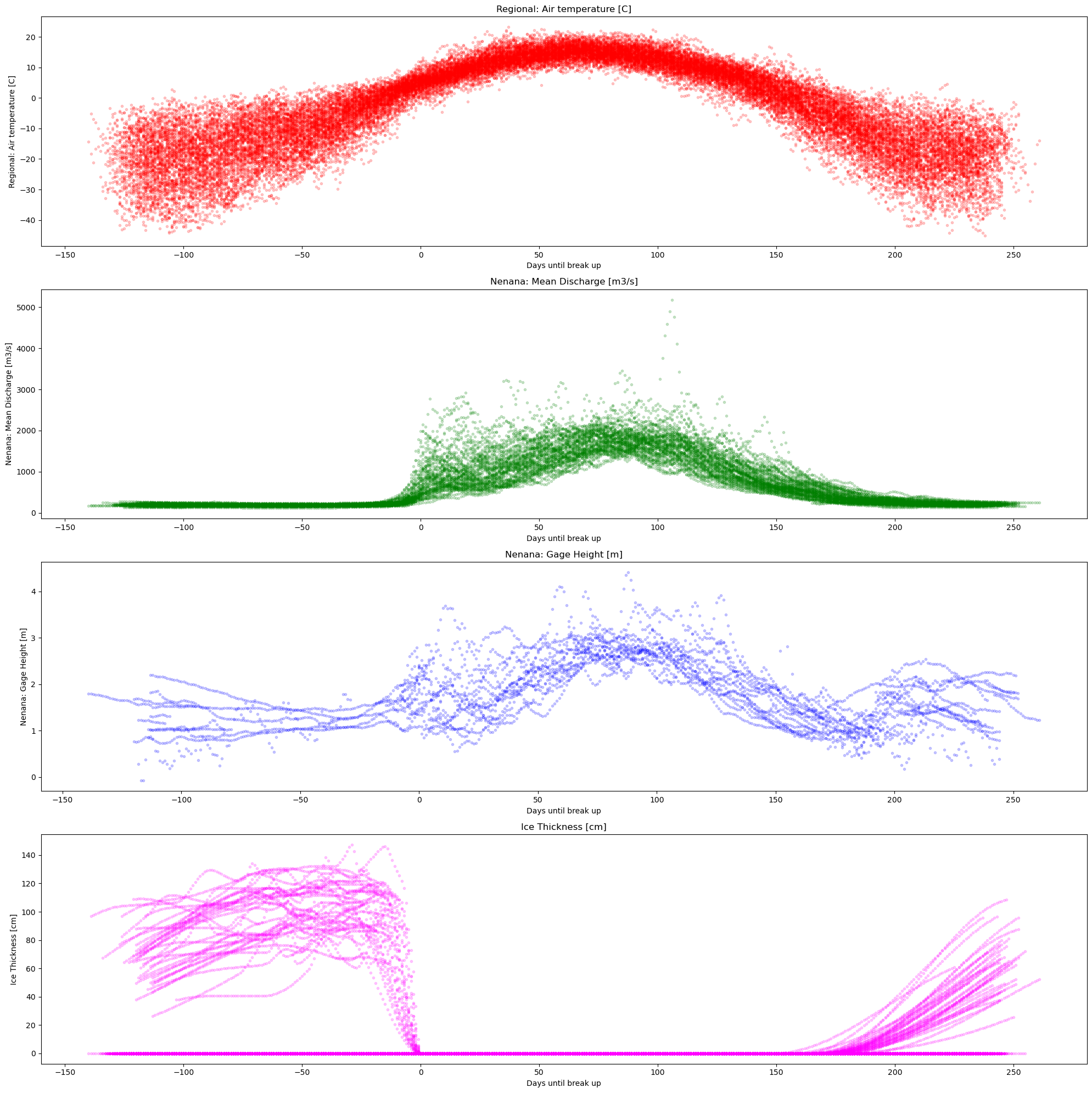
plot_contents(df_merged,
columns_to_plot=['Regional: Air temperature [C]','Nenana: Mean Discharge [m3/s]','Nenana: Gage Height [m]','Ice Thickness [cm]'], # what columns to plot, default all
col_cmap=['red','green','blue','magenta'], # list of colors for each column, default is sequential cmap, but list of colors can be passed as well
scatter_alpha=0.2, # we can 'mute' the scatter points if we choose lapha=0, then the col_map is irrelevant, cuz the scatter markers are no being plotted
plot_mean_std=False,
xaxis='Days until break up' , # we 'mute' the baseline across all years, similar here, if it were 'True' the color would have been grey'
multiyear=None, # we select which years to highlight
years_line_width=2, # change the iwth of line if necessary
plot_break_up_dates=False)
# we reload df cuz we need some column that we dropped at the beginning
Data=pd.read_csv("../../data/Time_series_DATA.txt",skiprows=149,index_col=0,sep='\t')
Data.index = pd.to_datetime(Data.index, format="%Y-%m-%d")
Data = Data[(Data.index.year >= 1917) & (Data.index.year < 2024)]
Data.info()
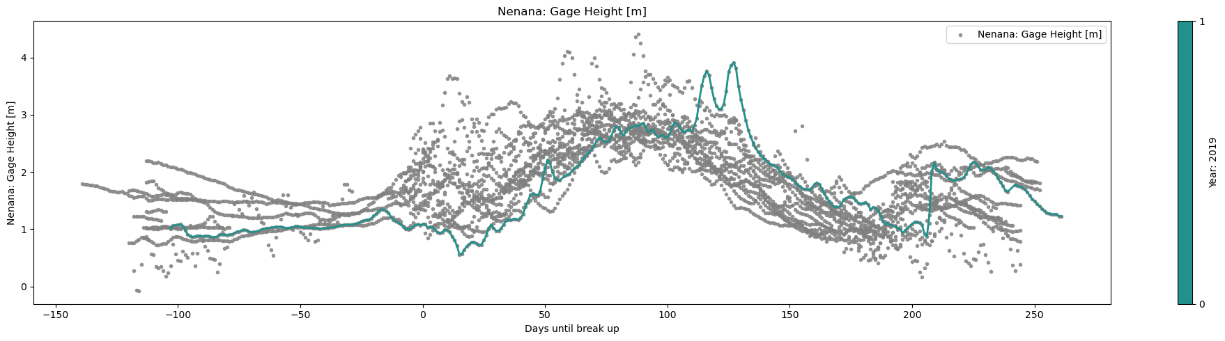
plot_contents(df_merged,
columns_to_plot=['Nenana: Gage Height [m]'], # what columns to plot, default all
col_cmap=['grey'], # list of colors for each column, default is sequential cmap, but list of colors can be passed as well
scatter_alpha=0.8, # we can 'mute' the scatter points if we choose lapha=0, then the col_map is irrelevant, cuz the scatter markers are no being plotted
plot_mean_std=False, # we 'mute' the baseline across all years, similar here, if it were 'True' the color would have been grey'
multiyear=[2019], # we select which years to highlight
years_line_width=2, # change the iwth of line if necessary
plot_break_up_dates=True,
xaxis='Days until break up') # plotting break_up_dates makers with annotations, default =False
<class 'pandas.core.frame.DataFrame'>
DatetimeIndex: 39081 entries, 1917-01-01 to 2023-12-31
Data columns (total 24 columns):
 #   Column                                             Non-Null Count  Dtype
---  ------                                             --------------  -----
 0   Regional: Air temperature [C]                      38563 non-null  float64
 1   Days since start of year                           38563 non-null  float64
 2   Days until break up                                38563 non-null  float64
 3   Nenana: Rainfall [mm]                              29516 non-null  float64
 4   Nenana: Snowfall [mm]                              19945 non-null  float64
 5   Nenana: Snow depth [mm]                            15984 non-null  float64
 6   Nenana: Mean water temperature [C]                 2418 non-null   float64
 7   Nenana: Mean Discharge [m3/s]                      22525 non-null  float64
 8   Nenana: Air temperature [C]                        31146 non-null  float64
 9   Fairbanks: Average wind speed [m/s]                9797 non-null   float64
 10  Fairbanks: Rainfall [mm]                           29586 non-null  float64
 11  Fairbanks: Snowfall [mm]                           29586 non-null  float64
 12  Fairbanks: Snow depth [mm]                         29555 non-null  float64
 13  Fairbanks: Air Temperature [C]                     29587 non-null  float64
 14  IceThickness [cm]                                  461 non-null    float64
 15  Regional: Solar Surface Irradiance [W/m2]          86 non-null     float64
 16  Regional: Cloud coverage [%]                       1272 non-null   float64
 17  Global: ENSO-Southern oscillation index            876 non-null    float64
 18  Gulkana Temperature [C]                            19146 non-null  float64
 19  Gulkana Precipitation [mm]                         18546 non-null  float64
 20  Gulkana: Glacier-wide winter mass balance [m.w.e]  58 non-null     float64
 21  Gulkana: Glacier-wide summer mass balance [m.w.e]  58 non-null     float64
 22  Global: Pacific decadal oscillation index          1284 non-null   float64
 23  Global: Artic oscillation index                    888 non-null    float64
dtypes: float64(24)
memory usage: 7.5 MB
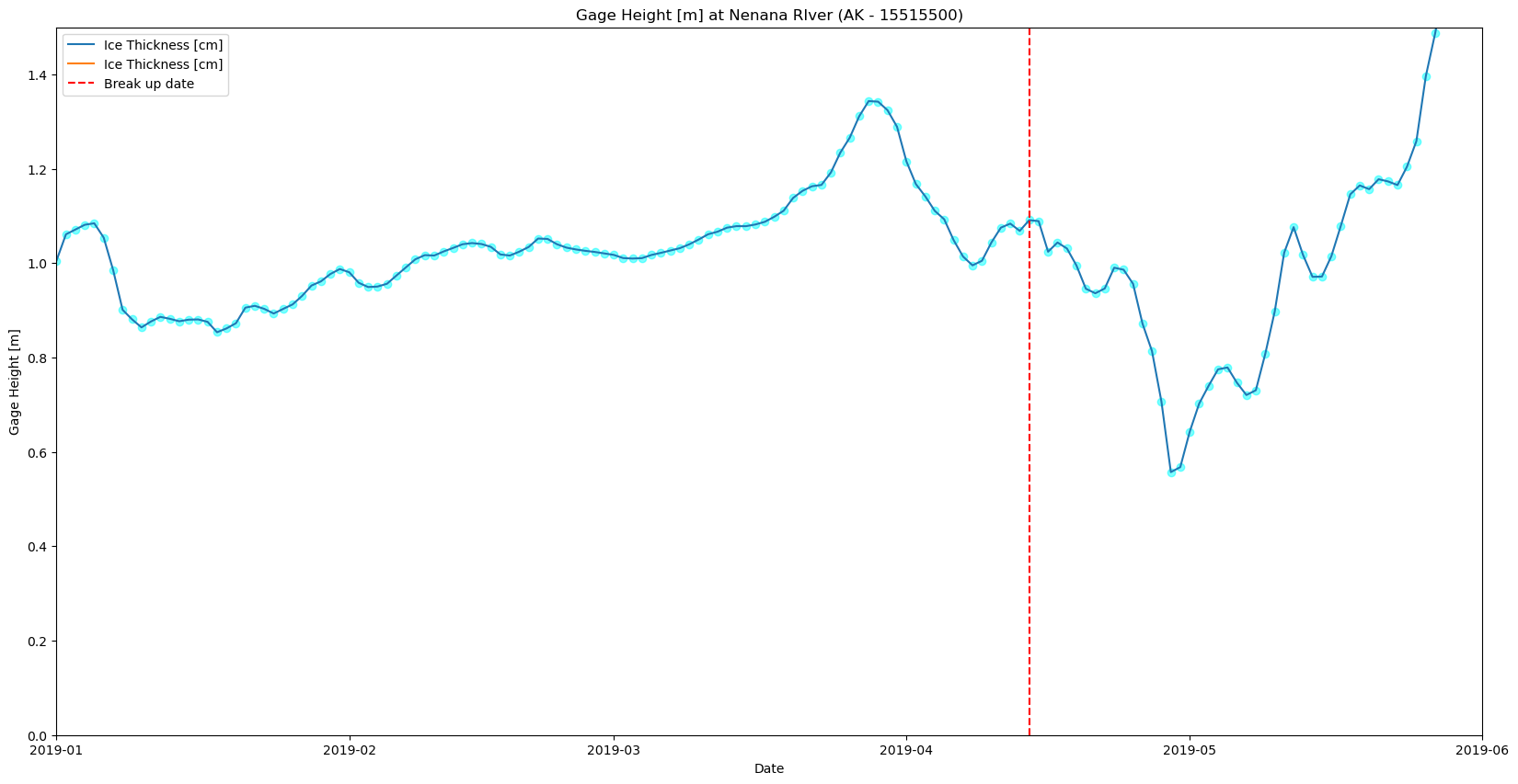
plt.figure(figsize=(20,10),)
plt.scatter(df_merged.index,df_merged['Nenana: Gage Height [m]'],color='cyan',marker='o',alpha=0.5)
plt.plot(df_merged.index,df_merged['Nenana: Gage Height [m]'],label='Ice Thickness [cm]')

plt.scatter(df_merged.index,df_merged['Nenana: Mean Discharge [m3/s]'],color='orange',marker='o',alpha=0.5)
plt.plot(df_merged.index,df_merged['Nenana: Mean Discharge [m3/s]'],label='Ice Thickness [cm]')
plt.xlim(pd.to_datetime(['2019/01/01','2019/06/01']))
plt.title('Gage Height [m] at Nenana RIver (AK - 15515500)')
plt.axvline(pd.to_datetime('2019-04-14'),color='red',linestyle='--',label='Break up date')
plt.ylim(0,1.5)
plt.xlabel('Date')
plt.ylabel('Gage Height [m]')
plt.legend()
plt.show()
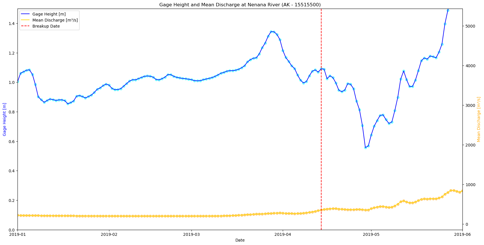
# Create figure and first axis
plt.figure(figsize=(20, 10))
ax1 = plt.gca()  # Get current axis

# Plot Gage Height on the first y-axis
ax1.scatter(df_merged.index, df_merged['Nenana: Gage Height [m]'], color='cyan', marker='o', alpha=0.5)
ax1.plot(df_merged.index, df_merged['Nenana: Gage Height [m]'], color='blue', label='Gage Height [m]')
ax1.set_ylabel('Gage Height [m]', color='blue')
ax1.set_ylim(0, 1.5)

# Create second y-axis for Discharge
ax2 = ax1.twinx()
ax2.scatter(df_merged.index, df_merged['Nenana: Mean Discharge [m3/s]'], color='orange', marker='o', alpha=0.5)
ax2.plot(df_merged.index, df_merged['Nenana: Mean Discharge [m3/s]'], color='gold', label='Mean Discharge [m³/s]')
ax2.set_ylabel('Mean Discharge [m³/s]', color='orange')

# Common settings
ax1.set_xlim(pd.to_datetime(['2019/01/01', '2019/06/01']))
plt.title('Gage Height and Mean Discharge at Nenana River (AK - 15515500)')
plt.axvline(pd.to_datetime('2019-04-14'), color='red', linestyle='--', label='Breakup Date')
ax1.set_xlabel('Date')

# Combine legends from both axes
lines, labels = ax1.get_legend_handles_labels()
lines2, labels2 = ax2.get_legend_handles_labels()
ax1.legend(lines + lines2, labels + labels2)

plt.show()
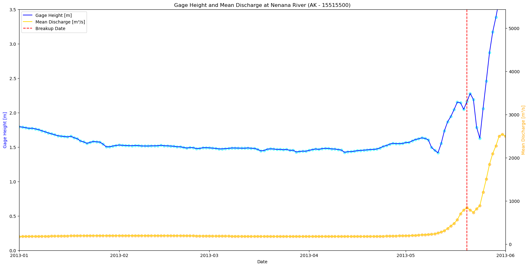
# Create figure and first axis
plt.figure(figsize=(20, 10))
ax1 = plt.gca()  # Get current axis

# Plot Gage Height on the first y-axis
ax1.scatter(df_merged.index, df_merged['Nenana: Gage Height [m]'], color='cyan', marker='o', alpha=0.5)
ax1.plot(df_merged.index, df_merged['Nenana: Gage Height [m]'], color='blue', label='Gage Height [m]')
ax1.set_ylabel('Gage Height [m]', color='blue')
ax1.set_ylim(0, 3.5)

# Create second y-axis for Discharge
ax2 = ax1.twinx()
ax2.scatter(df_merged.index, df_merged['Nenana: Mean Discharge [m3/s]'], color='orange', marker='o', alpha=0.5)
ax2.plot(df_merged.index, df_merged['Nenana: Mean Discharge [m3/s]'], color='gold', label='Mean Discharge [m³/s]')
ax2.set_ylabel('Mean Discharge [m³/s]', color='orange')

# Common settings
ax1.set_xlim(pd.to_datetime(['2013/01/01', '2013/06/01']))
plt.title('Gage Height and Mean Discharge at Nenana River (AK - 15515500)')
plt.axvline(pd.to_datetime('2013-05-20'), color='red', linestyle='--', label='Breakup Date')
ax1.set_xlabel('Date')

# Combine legends from both axes
lines, labels = ax1.get_legend_handles_labels()
lines2, labels2 = ax2.get_legend_handles_labels()
ax1.legend(lines + lines2, labels + labels2)

plt.show()
mask_2009 = (df_merged.index >= '2016-04-01') & (df_merged.index <= '2016-12-31')
df_merged.loc[mask_2009, 'Regional: Air temperature [C]'] = pd.NA
df_merged.loc[mask_2009, 'Nenana: Gage Height [m]'] = pd.NA
df_merged.loc[mask_2009, 'Nenana: Mean Discharge [m3/s]'] = pd.NA
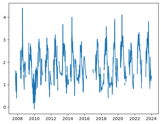
plt.plot(df_merged['Nenana: Gage Height [m]'], label='Regional: Air temperature [C]')
[<matplotlib.lines.Line2D at 0x1bb83b5f650>]
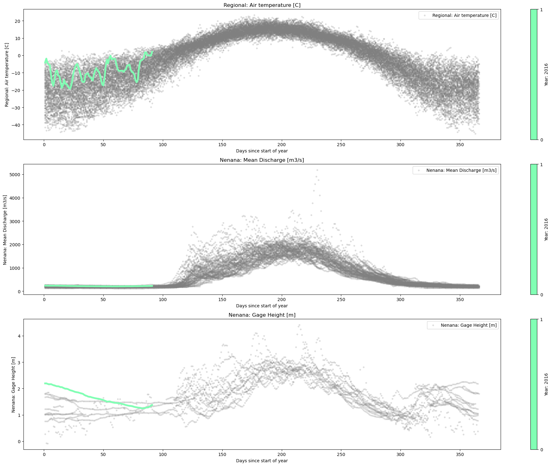
plot_contents(df_merged,
              columns_to_plot=['Regional: Air temperature [C]','Nenana: Mean Discharge [m3/s]','Nenana: Gage Height [m]'],     # what columns to plot, default all
              col_cmap=['grey'],                                     # list of colors for each column, default is sequential cmap, but list of colors can be passed as well
              scatter_alpha=0.2,                                     # we can 'mute' the scatter points if we choose lapha=0, then the col_map is irrelevant, cuz the scatter markers are no being plotted
              plot_mean_std=False,                                   # we 'mute' the baseline across all years, similar here, if it were 'True' the color would have been grey'
              multiyear=[2016],                            # we select which years to highlight
              years_line_width=4,                                    # change the iwth of line if necessary
              plot_break_up_dates=False,
              years_cmap='rainbow')                              # plotting break_up_dates makers with annotations, default =Fals)
Data.info()
<class 'pandas.core.frame.DataFrame'>
DatetimeIndex: 39081 entries, 1917-01-01 to 2023-12-31
Data columns (total 24 columns):
 #   Column                                             Non-Null Count  Dtype
---  ------                                             --------------  -----
 0   Regional: Air temperature [C]                      38563 non-null  float64
 1   Days since start of year                           38563 non-null  float64
 2   Days until break up                                38563 non-null  float64
 3   Nenana: Rainfall [mm]                              29516 non-null  float64
 4   Nenana: Snowfall [mm]                              19945 non-null  float64
 5   Nenana: Snow depth [mm]                            15984 non-null  float64
 6   Nenana: Mean water temperature [C]                 2418 non-null   float64
 7   Nenana: Mean Discharge [m3/s]                      22525 non-null  float64
 8   Nenana: Air temperature [C]                        31146 non-null  float64
 9   Fairbanks: Average wind speed [m/s]                9797 non-null   float64
 10  Fairbanks: Rainfall [mm]                           29586 non-null  float64
 11  Fairbanks: Snowfall [mm]                           29586 non-null  float64
 12  Fairbanks: Snow depth [mm]                         29555 non-null  float64
 13  Fairbanks: Air Temperature [C]                     29587 non-null  float64
 14  IceThickness [cm]                                  461 non-null    float64
 15  Regional: Solar Surface Irradiance [W/m2]          86 non-null     float64
 16  Regional: Cloud coverage [%]                       1272 non-null   float64
 17  Global: ENSO-Southern oscillation index            876 non-null    float64
 18  Gulkana Temperature [C]                            19146 non-null  float64
 19  Gulkana Precipitation [mm]                         18546 non-null  float64
 20  Gulkana: Glacier-wide winter mass balance [m.w.e]  58 non-null     float64
 21  Gulkana: Glacier-wide summer mass balance [m.w.e]  58 non-null     float64
 22  Global: Pacific decadal oscillation index          1284 non-null   float64
 23  Global: Artic oscillation index                    888 non-null    float64
dtypes: float64(24)
memory usage: 7.5 MB
import matplotlib.pyplot as plt
import pandas as pd
# Filter data for 2013 and 2019
df_2013 = df_merged[df_merged.index.year == 2013]
df_2019 = df_merged[df_merged.index.year == 2019]
df_2011 = df_merged[df_merged.index.year == 2016]
# Extract Month-Day format for the x-axis
df_2013['Month-Day'] = df_2013.index.strftime('%m-%d')
df_2019['Month-Day'] = df_2019.index.strftime('%m-%d')
# Create figure and first axis
plt.figure(figsize=(20, 10))
# Plot Gage Height on the first y-axis
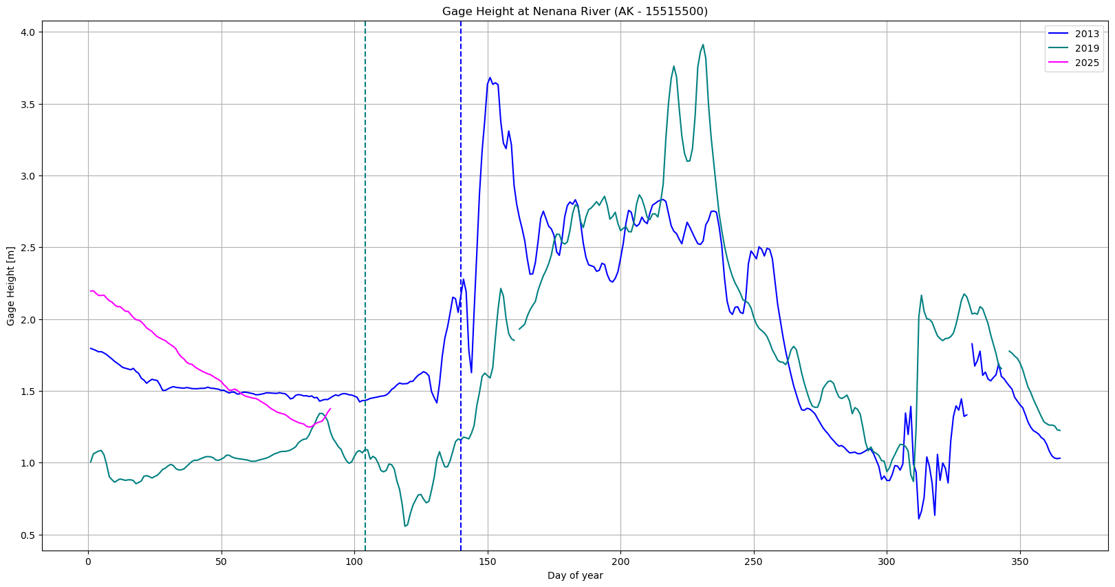
plt.plot(df_2013['Days since start of year'], df_2013['Nenana: Gage Height [m]'], color='blue', label='2013')
plt.plot(df_2019['Days since start of year'], df_2019['Nenana: Gage Height [m]'], color='teal', label='2019')
plt.plot(df_2011['Days since start of year'], df_2011['Nenana: Gage Height [m]'], color='magenta', label='2025')
plt.axvline(pd.to_datetime('2019-04-14').dayofyear,color='teal',linestyle='--')
plt.axvline(pd.to_datetime('2013-05-20').dayofyear,color='blue',linestyle='--')
plt.xlabel('Day of year')
# Common settings
plt.title('Gage Height at Nenana River (AK - 15515500)')
plt.ylabel('Gage Height [m]')
plt.grid(True)
plt.legend()
plt.show()
# Create figure and first axis
plt.figure(figsize=(20, 10))
# Plot Gage Height on the first y-axis
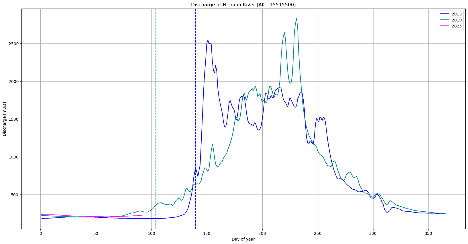
plt.plot(df_2013['Days since start of year'], df_2013['Nenana: Mean Discharge [m3/s]'], color='blue', label='2013')
plt.plot(df_2019['Days since start of year'], df_2019['Nenana: Mean Discharge [m3/s]'], color='teal', label='2019')
plt.plot(df_2011['Days since start of year'], df_2011['Nenana: Mean Discharge [m3/s]'], color='magenta', label='2025')
plt.axvline(pd.to_datetime('2019-04-14').dayofyear,color='teal',linestyle='--')
plt.axvline(pd.to_datetime('2013-05-20').dayofyear,color='blue',linestyle='--')
plt.xlabel('Day of year')
# Common settings
plt.title('Discharge at Nenana River (AK - 15515500)')
plt.ylabel('Discharge [m3/s]')
plt.grid(True)
plt.legend()
plt.show()
# Create figure and first axis
plt.figure(figsize=(20, 10))
# Plot Gage Height on the first y-axis
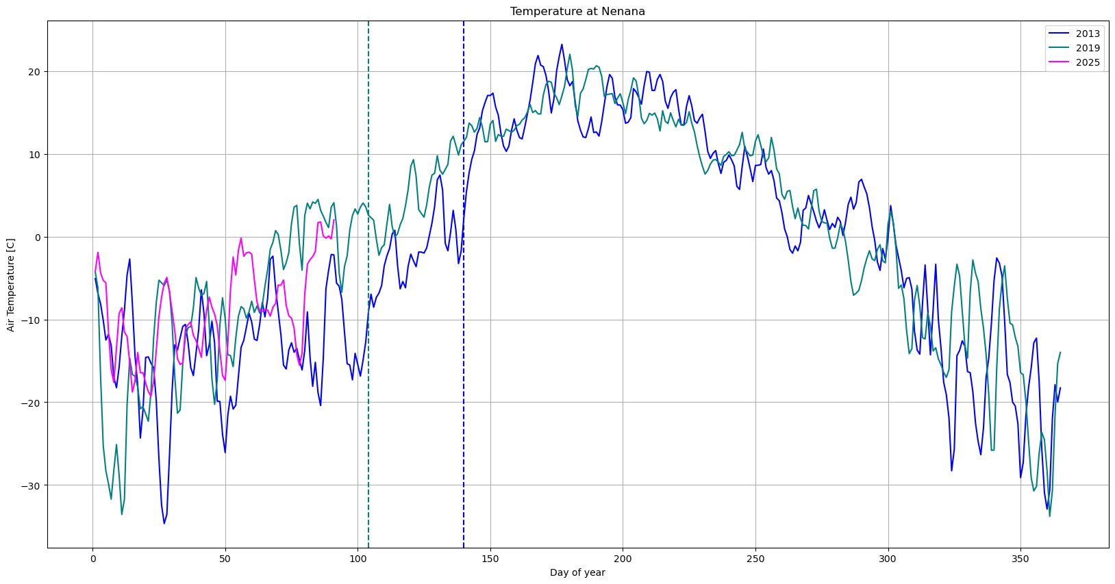
plt.plot(df_2013['Days since start of year'], df_2013['Regional: Air temperature [C]'], color='blue', label='2013')
plt.plot(df_2019['Days since start of year'], df_2019['Regional: Air temperature [C]'], color='teal', label='2019')
plt.plot(df_2011['Days since start of year'], df_2011['Regional: Air temperature [C]'], color='magenta', label='2025')
plt.axvline(pd.to_datetime('2019-04-14').dayofyear,color='teal',linestyle='--')
plt.axvline(pd.to_datetime('2013-05-20').dayofyear,color='blue',linestyle='--')
plt.xlabel('Day of year')
# Common settings
plt.title('Temperature at Nenana')
plt.ylabel('Air Temperature [C]')
plt.grid(True)
plt.legend()
plt.show()
C:\Users\gabri\AppData\Local\Temp\ipykernel_27920\164860991.py:10: SettingWithCopyWarning:
A value is trying to be set on a copy of a slice from a DataFrame.
Try using .loc[row_indexer,col_indexer] = value instead

See the caveats in the documentation: https://pandas.pydata.org/pandas-docs/stable/user_guide/indexing.html#returning-a-view-versus-a-copy
  df_2013['Month-Day'] = df_2013.index.strftime('%m-%d')
C:\Users\gabri\AppData\Local\Temp\ipykernel_27920\164860991.py:11: SettingWithCopyWarning:
A value is trying to be set on a copy of a slice from a DataFrame.
Try using .loc[row_indexer,col_indexer] = value instead

See the caveats in the documentation: https://pandas.pydata.org/pandas-docs/stable/user_guide/indexing.html#returning-a-view-versus-a-copy
  df_2019['Month-Day'] = df_2019.index.strftime('%m-%d')