Seasonal variations

Plotting the timeseries of the variables is useful to get a general insight about the historical variation and multiyear trends, but as you may noticed, most variables have a strong seasonal (yearly) component. The function plot_contents() can be use plot the seasonal variations of each year.

from funciones import*
import pandas as pd
import time
import matplotlib.pyplot as plt
import matplotlib.cm as cm
import numpy as np
import iceclassic as ice
file3=ice.import_data_browser('https://raw.githubusercontent.com/iceclassic/mude/main/book/data_files/time_serie_data.txt')
Data=pd.read_csv(file3,skiprows=162,index_col=0,sep='\t')   
Data.index = pd.to_datetime(Data.index, format="%Y-%m-%d")

Data = Data[Data.index.year < 2022]

Task 1:

Read the documentation for plot_contents() and plot the yearly variation of 'Regional: Air temperature [C]'and 'Gulkana Temperature [C]'

ice.plot_contents(Data,columns_to_plot=['Regional: Air temperature [C]','Gulkana Temperature [C]'],col_cmap='Paired',scatter_alpha=0.6)

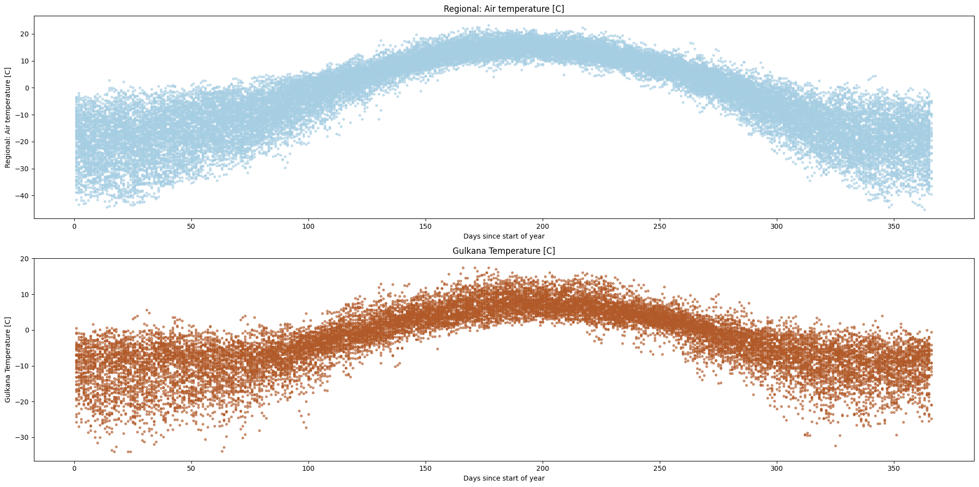
Using a scatter plot might not be the best idea as the figure can get cluttered, even when we adjust the opacity/size of the markers.
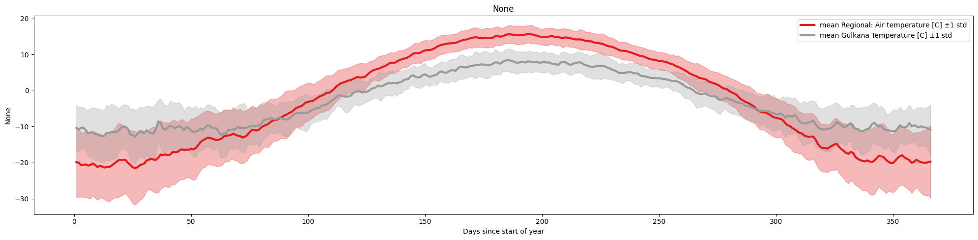
The figure becomes even less clear if we plot multiple variables/columns together. A simple alternative, is to plot the mean/standard deviation of each column, by passing the arguments plot_together=True, and plot_mean_std='only

ice.plot_contents(Data,columns_to_plot=['Regional: Air temperature [C]','Gulkana Temperature [C]'],plot_together=True,plot_mean_std='only',k=1)

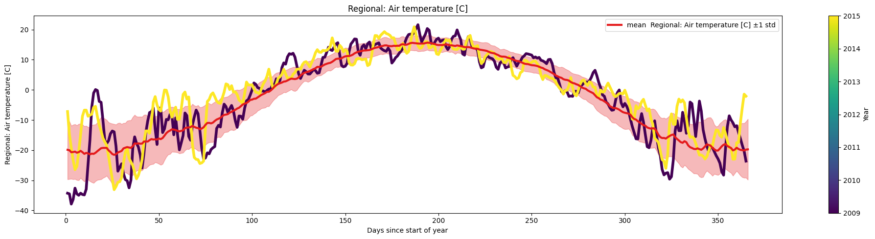
Another useful feature of the function is the ability to use it to compare the behavior of a certain set of years to the baseline ( aggregated data for all years)

Task 2:

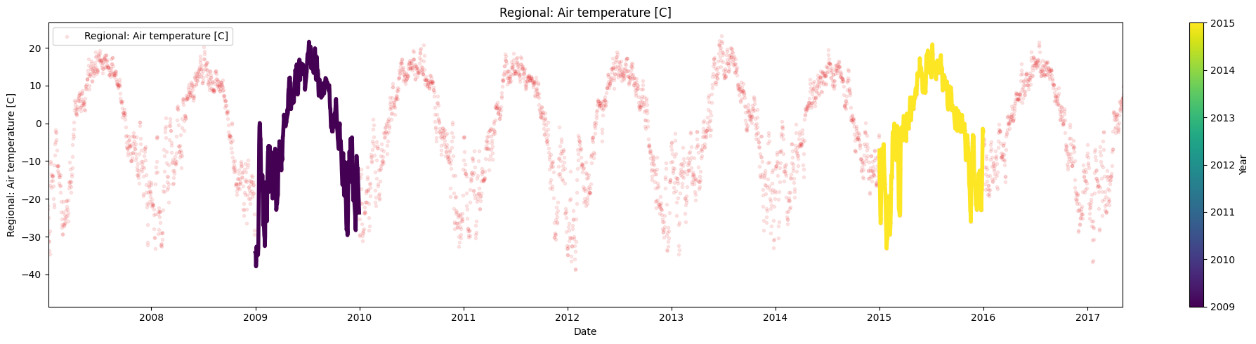
Use the argument multiyear to plot the data corresponding to the years 2009 and 2015 over the mean.

selected_years = [2009,2015]
ice.plot_contents(Data,k=1,plot_mean_std='only',multiyear=selected_years,columns_to_plot=['Regional: Air temperature [C]'])

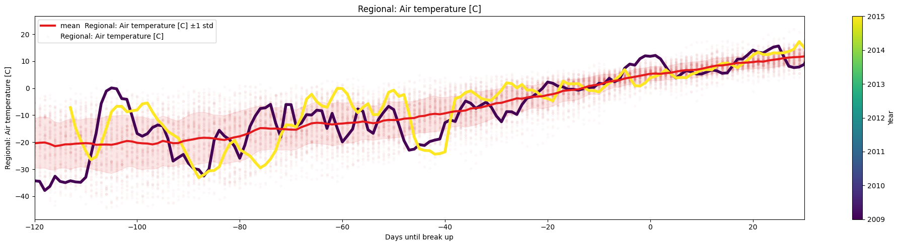
So far, we have used the number of days since the start of the year as the x-axis, which is a natural, yet completely arbitrary. More likely, another date or event/milestone is more meaningful, for example, choosing xaxis='Days until break-up' might be useful to observe trends leading up to the ice break-up, or , choosing xaxis='index' will recover the timeseries plot.

ice.plot_contents(Data,multiyear=selected_years,columns_to_plot=['Regional: Air temperature [C]'],xaxis='Days until break up',xlim=[-120,30],
              plot_mean_std='true',scatter_alpha=.02,std_alpha=.1) 

ice.plot_contents(Data,multiyear=selected_years,columns_to_plot=['Regional: Air temperature [C]'],xaxis='index',xlim=['2007/01/04','2017/05/03']) 

If we want to use an ‘x-axis’ that is not a column in the original DataFrame, we have to create a new DataFrame/Series, merge it to the original DataFrame and then use the previous function.

Task 3:

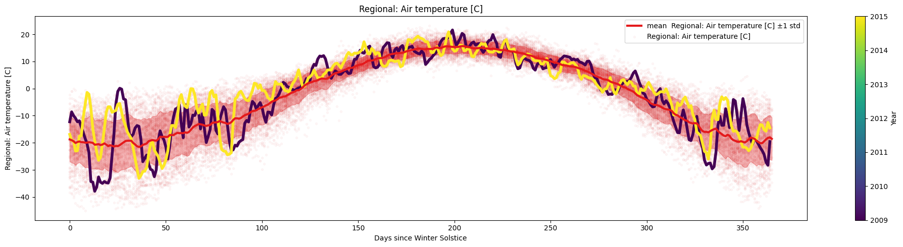
Use days_since_last_date() and plot_contents() to plot the temperature variation since the start of winter.

Data_2=days_since_last_date(Data,date='12/21',name='Winter Solstice')
ice.plot_contents(Data_2,k=1,plot_mean_std=True,columns_to_plot=['Regional: Air temperature [C]'],xaxis='Winter Solstice',xaxis_name='Days since Winter Solstice',scatter_alpha=0.03,multiyear=selected_years)

groupby and transform

So far we have grouped variables using the number of days since the last occurrence of a date (‘MM/DD’), but for more complex groupings it is convenient to use groupby and transform instead.

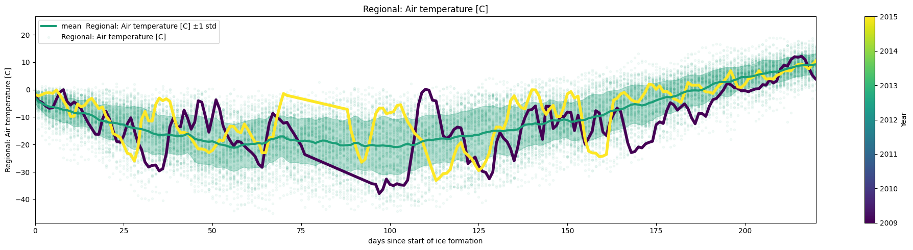
For example, lets try to re-create the plot above but considering the ‘number of days since the river began to freeze’ which happens at different dates each year.

Let’s define the event: river has began to freeze as the latest occasion( in the year) since the mean daily temperature was below zero for three consecutive days after it was above 0.

Naive Approach

A simple approach would be to loop through each year and day checking if the river has started to freeze.

Task 4:

Complete the missing line int the following code snippet, use the time module to estimate the time needed to execute the operation.

t1_0 = time.time()
years = Data.index.year.unique()
freezing_dates_1 = [None] * len(years)  

for year_index, year in enumerate(years):  # Looping through years 
    df_year = Data[Data.index.year == year].copy()  # Extracting data for that year
    df_year['Rolling Mean'] = df_year['Regional: Air temperature [C]'].rolling(window=3).mean()  # Compute rolling mean

    Frozen = False  # Initial state

    for i in range(3, len(df_year)):  # Looping through days of that year, starting from day 3 since we are using a rolling mean of 3
        T_current = df_year.at[df_year.index[i], 'Regional: Air temperature [C]']  
        T_rolling_mean = df_year.at[df_year.index[i], 'Rolling Mean']  
        T_rolling_mean_prev = df_year.at[df_year.index[i - 1], 'Rolling Mean']  
        
        if T_rolling_mean < 0 and T_rolling_mean_prev >= 0:  # Condition for freezing
            Frozen = True
            freezing_dates_1[year_index] = df_year.index[i].strftime('%Y/%m/%d')  

t1_f = time.time()  # Record the end time
delta_t1 = t1_f - t1_0
print(f"Elapsed time: {delta_t1:.4f} seconds")

Elapsed time: 1.3430 seconds

Vector approach

The method .groupby() is used to split the dataframe into groups based on some criteria, then the method .transform() applies a function to the group.

Depending on the characteristics of the DataFrame/Series and the operation that you want to apply, similar methods such as .filter(), . apply(), .agg() or .map() might be more suitable (see user guide),

t2_0 = time.time()
rolling_avg_below_zero = Data['Regional: Air temperature [C]'].rolling(window=3).mean().lt(0) # rolling mean '.ls'= less than and returns boolean
freezing_dates_2 = (
    rolling_avg_below_zero.groupby(Data.index.year)                                            # Group by year
    .apply(lambda x: x.index[x & ~x.shift(1, fill_value=False)].max())                         # logic to find the date and then keep the max date of each group(year)                       
    .dropna()                                                                                  # To avoid errors  in next line when the condition is not met
    .apply(lambda date: date.strftime('%Y/%m/%d'))                                             # Convert to string every element                                   
    .tolist()                                                                                  # Convert to list       
)
t2_f = time.time()  # Record the end time
delta_t2 = t2_f - t2_0
print(f"Elapsed time: {delta_t2:.4f} seconds")

Elapsed time: 0.0340 seconds

In the code above we did not use a function per se, instead we used a lambda expression. Lambda expression are temporary and anonymous functions, that allows us to evaluate a logical expression in a single line, without necessary defining the function .

The vector approach is generally faster and more flexible as multiple methods and expressions can be efficiently apply to each group. However, it can be a little difficult to understand if you are not familiar with the syntax. The code above consist of 5 steps.

1. We create a Series with the freezing condition.

   • .rolling(window=3) groups the data corresponding to three consecutive element. Because our index are dates, we are grouping the date of three consecutive days

   • .mean() computes the mean of the grouped data

   • .lt(0) decide if the mean of the grouped is less than (lt) 0. This logical expression output a boolean

2. Grouping the data

   • .groupby(Data.index.year) groups the element of the Series according to the year in Data

   • .index.year extracts the year attribute of the datetime index to use the year of each row to group the data

3. Identifies when the freezing condition changes

   • apply(lambda x: ): defines that we will use a lambda expression with xthe variable

   • x & ~x.shift(1, fill_value=False) Use the logical operator AND (&) to compare the variable with the negated (~) shifted variable.

   • x.shift(1, fill_value=False)shift the variable by one position, and assigning False to the first position.

4. Identifies the latest instance of change of freezing condition in each year

   • x.index[] get the date associated with the change of freezing conditions

   • .max() get the latest date in each year ( maximum value of the index in the group (the data is grouped by year))

5. Post Processing

   • .dropna() drop the empty values which correspond to years where the freezing condition never happened (in this parituclar case it correspond to year without temperature data)

   • .apply(lambda date: date.strftime('%Y/%m/%d')) format the datetime object to a string

   • .tolist() convert the Series to a list

print(freezing_dates_1)
print(freezing_dates_2)
Data=days_since_last_date(Data,date=freezing_dates_2,name='days since start of ice formation')
ice.plot_contents(Data,plot_mean_std=True,multiyear=selected_years,columns_to_plot=['Regional: Air temperature [C]'],
              xaxis='days since start of ice formation',scatter_alpha=0.05,col_cmap='Dark2',k=1,xlim=[0,220])

[None, None, None, None, None, None, None, None, None, None, None, None, None, None, None, None, '1917/10/15', '1918/10/14', '1919/10/29', '1920/10/02', '1921/10/13', '1922/10/19', '1923/10/31', '1924/10/07', '1925/10/23', '1926/10/25', '1927/10/05', '1928/11/06', '1929/10/13', '1930/10/11', '1931/10/10', '1932/10/14', '1933/10/04', '1934/12/10', '1935/11/06', '1936/10/28', '1937/10/18', '1938/10/28', '1939/10/05', '1940/10/30', '1941/10/09', '1942/10/07', '1943/10/20', '1944/10/22', '1945/10/08', '1946/10/19', '1947/10/10', '1948/10/06', '1949/10/05', '1950/10/10', '1951/11/04', '1952/10/18', '1953/10/17', '1954/11/04', '1955/10/08', '1956/09/22', '1957/10/25', '1958/10/04', '1959/10/07', '1960/10/07', '1961/10/23', '1962/10/18', '1963/10/10', '1964/10/15', '1965/09/30', '1966/10/09', '1967/10/06', '1968/10/05', '1969/10/20', '1970/11/03', '1971/10/19', '1972/10/20', '1973/10/06', '1974/09/30', '1975/10/08', '1976/11/15', '1977/10/13', '1978/10/11', '1979/11/13', '1980/10/27', '1981/10/27', '1982/10/03', '1983/10/14', '1984/10/10', '1985/10/12', '1986/10/16', '1987/10/26', '1988/10/06', '1989/10/10', '1990/10/13', '1991/10/08', '1992/10/09', '1993/10/18', '1994/10/08', '1995/10/11', '1996/09/29', '1997/11/12', '1998/10/01', '1999/10/06', '2000/10/17', '2001/10/11', '2002/11/07', '2003/10/13', '2004/10/14', '2005/10/09', '2006/10/14', '2007/10/04', '2008/09/28', '2009/10/16', '2010/10/09', '2011/10/18', '2012/10/11', '2013/10/31', '2014/10/05', '2015/10/21', '2016/10/15', '2017/10/31', '2018/10/28', '2019/10/31', '2020/10/12', '2021/10/12']
['1917/10/15', '1918/10/14', '1919/10/29', '1920/10/02', '1921/10/13', '1922/10/19', '1923/10/31', '1924/10/07', '1925/10/23', '1926/10/25', '1927/10/05', '1928/11/06', '1929/10/13', '1930/10/11', '1931/10/10', '1932/10/14', '1933/10/04', '1934/12/10', '1935/11/06', '1936/10/28', '1937/10/18', '1938/10/28', '1939/10/05', '1940/10/30', '1941/10/09', '1942/10/07', '1943/10/20', '1944/10/22', '1945/10/08', '1946/10/19', '1947/10/10', '1948/10/06', '1949/10/05', '1950/10/10', '1951/11/04', '1952/10/18', '1953/10/17', '1954/11/04', '1955/10/08', '1956/09/22', '1957/10/25', '1958/10/04', '1959/10/07', '1960/10/07', '1961/10/23', '1962/10/18', '1963/10/10', '1964/10/15', '1965/09/30', '1966/10/09', '1967/10/06', '1968/10/05', '1969/10/20', '1970/11/03', '1971/10/19', '1972/10/20', '1973/10/06', '1974/09/30', '1975/10/08', '1976/11/15', '1977/10/13', '1978/10/11', '1979/11/13', '1980/10/27', '1981/10/27', '1982/10/03', '1983/10/14', '1984/10/10', '1985/10/12', '1986/10/16', '1987/10/26', '1988/10/06', '1989/10/10', '1990/10/13', '1991/10/08', '1992/10/09', '1993/10/18', '1994/10/08', '1995/10/11', '1996/09/29', '1997/11/12', '1998/10/01', '1999/10/06', '2000/10/17', '2001/10/11', '2002/11/07', '2003/10/13', '2004/10/14', '2005/10/09', '2006/10/14', '2007/10/04', '2008/09/28', '2009/10/16', '2010/10/09', '2011/10/18', '2012/10/11', '2013/10/31', '2014/10/05', '2015/10/21', '2016/10/15', '2017/10/31', '2018/10/28', '2019/10/31', '2020/10/12', '2021/10/12']

Task 5:

Use groupby() and transform() to add a column with the accumulated number of days that the temperature has been over -2 degree. And another column with the cumulative sum of the difference between the temperature and -2 [C], ignore the days that had negative temperature (i.e only days where the mean temperature was positive ( use masks(), clip() or use just logic))

Data['days_over_one'] = Data.groupby(Data.index.year)['Regional: Air temperature [C]'].transform(lambda x: (x > -2).cumsum()) # assumes that the number of day over 1 since the start of ice formation to jan 01 is zero 
Data['cumsum_pos_temp'] = Data.groupby(Data.index.year)['Regional: Air temperature [C]'].transform(lambda x: x.clip(lower=0).where(x > -2).cumsum())